frd

주파수 응답 데이터 모델

설명

frd를 사용하여, 실수 값 또는 복소수 값을 갖는 주파수 응답 데이터 모델을 만들거나 동적 시스템 모델을 주파수 응답 데이터 모델 형식으로 변환합니다.

주파수 응답 데이터 모델은 복소수 주파수 응답 데이터를 그에 대응하는 주파수 지점과 함께 저장합니다. 예를 들어 주파수 응답 데이터 모델 H(jw_i)는 각 입력 주파수 w_i에서의 주파수 응답을 저장합니다. 여기서 i = 1,…,n입니다. frd 모델 객체는 연속시간 또는 이산시간에서 SISO 또는 MIMO 주파수 응답 데이터 모델을 표현할 수 있습니다. 자세한 내용은 Frequency Response Data (FRD) Models 항목을 참조하십시오.

frd를 사용하여 일반화된 주파수 응답 데이터(genfrd) 모델을 만들 수도 있습니다.

생성

frd 모델은 다음 방법 중 하나로 얻을 수 있습니다.

frd 명령을 사용하여 주파수 응답 데이터에서 모델을 만듭니다. 예를 들어, 특정 주파수에서 가져온 주파수 응답 데이터를 사용하여 frd 모델을 만들 수 있습니다.
예제는 SISO 주파수 응답 데이터 모델 항목을 참조하십시오.
지정된 주파수에서의 모델 주파수 응답을 계산하여 ss 모델 같은 선형 모델을 frd 모델로 변환합니다.
예제는 상태공간 모델을 주파수 응답 데이터 모델로 변환하기 항목을 참조하십시오.
오프라인 주파수 응답 추정 워크플로를 사용하여 모델을 추정합니다. 이러한 워크플로에는 Simulink^®Control Design™이 필요합니다.
자세한 내용은 Estimate Frequency Response at the Command Line (Simulink Control Design) 항목과 Estimate Frequency Response Using Model Linearizer (Simulink Control Design) 항목을 참조하십시오.

구문

sys = frd(response,frequency)

sys = frd(response,frequency,ts)

sys = frd(response,frequency,ltiSys)

sys = frd(___,Name,Value)

sys = frd(ltiSys,frequency)

sys = frd(ltiSys,frequency,FrequencyUnits)

설명

sys = frd(response,frequency)는 ResponseData 및 Frequency 속성을 설정하여 연속시간 주파수 응답 데이터(frd) 모델을 만듭니다. frequency에는 음수 주파수와 양수 주파수가 모두 포함될 수 있습니다.

예제

sys = frd(response,frequency,ts)는 샘플 시간이 ts인 이산시간 frd 모델을 만듭니다. 샘플 시간을 지정하지 않은 상태로 두려면 ts를 –1로 설정하십시오.

예제

sys = frd(response,frequency,ltiSys)는 샘플 시간을 비롯해 동적 시스템 모델 ltiSys에서 상속한 속성을 사용하여 주파수 응답 데이터 모델을 만듭니다.

예제

sys = frd(___,Name,Value)는 위에 열거된 입력 인수 조합에 대해 하나 이상의 이름-값 인수를 사용하여 주파수 응답 데이터 모델의 속성을 설정합니다.

예제

sys = frd(ltiSys,frequency)는 동적 시스템 모델 ltiSys를 주파수 응답 데이터 모델로 변환합니다. frd는 frequency로 지정된 주파수에서의 주파수 응답을 계산합니다. sys는 ltiSys.TimeUnit에서 주파수 단위 rad/TimeUnit을 상속합니다.

예제

sys = frd(ltiSys,frequency,FrequencyUnits)는 FrequencyUnit으로 지정된 단위로 주파수를 해석합니다.

입력 인수

모두 확장

`response` — 주파수 응답 데이터
벡터 | 다차원 배열

주파수 응답 데이터로, 복소수로 구성된 벡터 또는 다차원 배열로 지정됩니다.

SISO 시스템의 경우 frequency에 지정된 주파수 지점에서의 주파수 응답 값으로 구성된 벡터를 지정하십시오.
Nu개 입력과 Ny개 출력을 갖는 MIMO 시스템의 경우 Ny×Nu×Nf 배열을 지정하십시오. 여기서 Nf는 주파수 지점 개수입니다.
Nu개 입력과 Ny개 출력을 갖는 모델로 구성된 S1×...×Sn 배열의 경우 크기가 [Ny Nu Nf S1 … Sn]인 다차원 배열을 지정하십시오.
예를 들어 크기가 [Ny,Nu,Nf,3,4]인 response는 모델로 구성된 3×4 배열에 대한 응답 데이터를 나타냅니다. 각 모델에는 Ny개의 출력, Nu개의 입력, Nf개의 주파수 지점이 있습니다.

이 입력은 ResponseData 속성을 설정합니다.

`frequency` — 주파수 지점
벡터

response에 대응하는 주파수 지점으로, Nf개 지점을 포함하는 벡터로 지정됩니다. frequency에는 양수 주파수와 음수 주파수가 모두 포함될 수 있습니다.

이 입력은 Frequency 속성을 설정합니다.

`ts` — 샘플 시간
스칼라

샘플 시간으로, 스칼라로 지정됩니다.

이 입력은 Ts 속성을 설정합니다.

`ltiSys` — 동적 시스템
동적 시스템 모델 | 모델 배열

동적 시스템으로, SISO 또는 MIMO 동적 시스템 모델로 지정되거나 동적 시스템 모델로 구성된 배열로 지정됩니다. 사용 가능한 동적 시스템에는 다음이 포함됩니다.

연속시간 또는 이산시간 수치적 LTI 모델(예: tf, zpk, ss 또는 pid 모델).
일반화된 LTI 모델 또는 불확실 LTI 모델(예: genss, uss (Robust Control Toolbox) 모델). (불확실 모델을 사용하려면 Robust Control Toolbox™가 필요합니다.)
그 결과로 얻은 frd 모델은 다음을 가정합니다.
- 조정 가능한 제어 설계 블록의 경우 조정 가능한 컴포넌트의 현재 값
- 불확실한 제어 설계 블록의 경우 공칭 모델 값
식별된 LTI 모델(예: idtf (System Identification Toolbox), idss (System Identification Toolbox), idproc (System Identification Toolbox), idpoly (System Identification Toolbox) 또는 idgrey (System Identification Toolbox) 모델). (식별된 모델을 사용하려면 System Identification Toolbox™가 필요합니다.)

속성

모두 확장

`ResponseData` — 주파수 응답 데이터
복소수로 구성된 다차원 배열

주파수 응답 데이터로, 복소수로 구성된 다차원 배열로 지정됩니다.

SISO 시스템의 경우 ResponseData는 Frequency 속성에 지정된 Nf개 주파수 지점에서의 주파수 응답 값으로 구성된 1×1×Nf 배열입니다.
Nu개 입력과 Ny개 출력을 갖는 MIMO 시스템의 경우 ResponseData는 Ny×Nu×Nf 배열입니다. 여기서 Nf는 주파수 지점 개수입니다.
예를 들어 ResponseData(ky,ku,kf)는 주파수 Frequency(kf)에서 입력 ku부터 출력 ky까지의 주파수 응답을 나타냅니다.
Nu개 입력과 Ny개 출력을 갖는 모델들로 구성된 S1×...×Sn 배열의 경우 ResponseData는 크기가 [Ny Nu Nf S1 … Sn]인 다차원 배열입니다.
예를 들어 크기가 [Ny,Nu,Nf,3,4]인 ResponseData는 모델로 구성된 3×4 배열에 대한 응답 데이터를 나타냅니다. 각 모델에는 Ny개의 출력, Nu개의 입력, Nf개의 주파수 지점이 있습니다.

`Frequency` — 주파수 지점
벡터

ResponseData에 대응하는 주파수 지점으로, Nf개 지점을 포함하는 벡터로 지정됩니다(단위: FrequencyUnit으로 지정됨).

`FrequencyUnit` — 주파수 벡터의 단위
`'rad/TimeUnit'` (디폴트 값) | `'cycles/TimeUnit'` | `'rad/s'` | `'Hz'` | `'kHz'` | `'MHz'` | `'GHz'` | `'rpm'`

Frequency 속성에 지정된 주파수 벡터의 단위로, 다음 값 중 하나로 지정됩니다.

'rad/TimeUnit'
'cycles/TimeUnit'
'rad/s'
'Hz'
'kHz'
'MHz'
'GHz'
'rpm'

단위 'rad/TimeUnit'과 'cycles/TimeUnit'은 TimeUnit 속성에 지정된 시간 단위를 기준으로 합니다.

이 속성을 변경해도 데이터가 리샘플링되거나 변환되지 않습니다. 속성을 수정하면 기존 데이터의 해석만 변경됩니다. 데이터를 다른 주파수 단위로 변환하려면 chgFreqUnit을 사용하십시오.

`IODelay` — 전송 지연
`0` (디폴트 값) | 스칼라 | `Ny`×`Nu` 배열

전송 지연으로, 다음 중 하나로 지정됩니다.

스칼라 — SISO 시스템에 대한 전송 지연을 지정하거나 MIMO 시스템의 모든 입력/출력 쌍에 대해 동일한 전송 지연을 지정합니다.
Ny×Nu 배열 — MIMO 시스템의 각 입력/출력 쌍에 대해 개별적인 전송 지연을 지정합니다. 여기서 Ny는 출력의 개수이고 Nu는 입력의 개수입니다.

연속시간 시스템의 경우 TimeUnit 속성으로 지정된 시간 단위로 전송 지연을 지정합니다. 이산시간 시스템의 경우 샘플 시간 Ts의 정수 배로 전송 지연을 지정합니다.

`InputDelay` — 입력 지연
`0` (디폴트 값) | 스칼라 | `Nu`×1 벡터

각 입력 채널에 대한 입력 지연으로, 다음 중 하나로 지정됩니다.

스칼라 — SISO 시스템에 대한 입력 지연을 지정하거나 다중 입력 시스템의 모든 입력에 대해 동일한 지연을 지정합니다.
Nu×1 벡터 — 다중 입력 시스템의 입력에 대해 개별적인 입력 지연을 지정합니다. 여기서 Nu는 입력의 개수입니다.

연속시간 시스템의 경우 TimeUnit 속성으로 지정된 시간 단위로 입력 지연을 지정합니다. 이산시간 시스템의 경우 샘플 시간 Ts의 정수 배로 입력 지연을 지정합니다.

자세한 내용은 선형 시스템의 시간 지연 항목을 참조하십시오.

`OutputDelay` — 출력 지연
`0` (디폴트 값) | 스칼라 | `Ny`×1 벡터

각 출력 채널에 대한 출력 지연으로, 다음 중 하나로 지정됩니다.

스칼라 — SISO 시스템에 대한 출력 지연을 지정하거나 다중 출력 시스템의 모든 출력에 대해 동일한 지연을 지정합니다.
Ny×1 벡터 — 다중 출력 시스템의 출력에 대해 개별적인 출력 지연을 지정합니다. 여기서 Ny는 출력의 개수입니다.

연속시간 시스템의 경우 TimeUnit 속성으로 지정된 시간 단위로 출력 지연을 지정합니다. 이산시간 시스템의 경우 샘플 시간 Ts의 정수 배로 출력 지연을 지정합니다.

자세한 내용은 선형 시스템의 시간 지연 항목을 참조하십시오.

`Ts` — 샘플 시간
`0` (디폴트 값) | 양의 스칼라 | `-1`

샘플 시간으로, 다음으로 지정됩니다.

연속시간 시스템의 경우 0.
이산시간 시스템의 샘플링 주기를 나타내는 양의 스칼라. Ts를 TimeUnit 속성으로 지정된 시간 단위로 지정합니다.
샘플 시간이 지정되지 않은 이산시간 시스템의 경우 -1.

참고

Ts를 변경해도 모델이 이산화되거나 리샘플링되지 않습니다.

`TimeUnit` — 시간 변수 단위
`'seconds'` (디폴트 값) | `'nanoseconds'` | `'microseconds'` | `'milliseconds'` | `'minutes'` | `'hours'` | `'days'` | `'weeks'` | `'months'` | `'years'` | ...

시간 변수 단위로, 다음 중 하나로 지정됩니다.

'nanoseconds'
'microseconds'
'milliseconds'
'seconds'
'minutes'
'hours'
'days'
'weeks'
'months'
'years'

TimeUnit을 변경해도 다른 속성에 영향을 미치지 않으나 전체적인 시스템 동작이 변경됩니다. 시스템 동작을 수정하지 않고 시간 단위 간 변환을 수행하려면 chgTimeUnit을 사용하십시오.

`InputName` — 입력 채널 이름
`''` (디폴트 값) | 문자형 벡터 | 문자형 벡터로 구성된 셀형 배열

입력 채널 이름으로, 다음 중 하나로 지정됩니다.

단일 입력 모델의 경우 문자형 벡터.
다중 입력 모델의 경우 문자형 벡터로 구성된 셀형 배열.
입력 채널에 대해 지정된 이름이 없는 경우 ''.

또는 자동 벡터 확장을 사용하여 다중 입력 모델에 입력 이름을 할당할 수 있습니다. 예를 들어, sys가 2-입력 모델인 경우 다음을 입력합니다.

sys.InputName = 'controls';

입력 이름이 자동으로 {'controls(1)';'controls(2)'}로 확장됩니다.

축약 표기법 u를 사용하여 InputName 속성을 참조할 수 있습니다. 예를 들어, sys.u는 sys.InputName과 동일합니다.

InputName을 사용하여 다음을 수행할 수 있습니다.

모델 표시 화면과 플롯에서 채널 식별.
MIMO 시스템의 서브시스템 추출.
모델 상호 연결 시 연결 점 지정.

`InputUnit` — 입력 채널 단위
`''` (디폴트 값) | 문자형 벡터 | 문자형 벡터로 구성된 셀형 배열

입력 채널 단위로, 다음 중 하나로 지정됩니다.

단일 입력 모델의 경우 문자형 벡터.
다중 입력 모델의 경우 문자형 벡터로 구성된 셀형 배열.
입력 채널에 대해 지정된 단위가 없는 경우 ''.

InputUnit을 사용하여 입력 신호 단위를 지정합니다. InputUnit은 시스템 동작에 영향을 미치지 않습니다.

`InputGroup` — 입력 채널 그룹
구조체

입력 채널 그룹으로, 구조체로 지정됩니다. InputGroup을 사용하여 MIMO 시스템의 입력 채널을 그룹으로 할당하고 각 그룹을 이름으로 참조할 수 있습니다. InputGroup의 필드 이름은 그룹 이름이고 필드 값은 각 그룹의 입력 채널입니다. 예를 들어 다음을 입력하여 각각 입력 채널 1, 2와 입력 채널 3, 5를 포함하는 controls와 noise라는 입력 그룹을 만듭니다.

sys.InputGroup.controls = [1 2];
sys.InputGroup.noise = [3 5];

이때 다음을 사용하여 controls 입력에서 모든 출력으로 서브시스템을 추출할 수 있습니다.

sys(:,'controls')

기본적으로 InputGroup은 필드가 없는 구조체입니다.

`OutputName` — 출력 채널 이름
`''` (디폴트 값) | 문자형 벡터 | 문자형 벡터로 구성된 셀형 배열

출력 채널 이름으로, 다음 중 하나로 지정됩니다.

단일 출력 모델의 경우 문자형 벡터.
다중 출력 모델의 경우 문자형 벡터로 구성된 셀형 배열.
출력 채널에 대해 지정된 이름이 없는 경우 ''.

또는 자동 벡터 확장을 사용하여 다중 출력 모델에 출력 이름을 할당할 수 있습니다. 예를 들어, sys가 2-출력 모델인 경우 다음을 입력합니다.

sys.OutputName = 'measurements';

출력 이름이 자동으로 {'measurements(1)';'measurements(2)'}로 확장됩니다.

축약 표기법 y를 사용하여 OutputName 속성을 참조할 수도 있습니다. 예를 들어, sys.y는 sys.OutputName과 동일합니다.

OutputName을 사용하여 다음을 수행할 수 있습니다.

모델 표시 화면과 플롯에서 채널 식별.
MIMO 시스템의 서브시스템 추출.
모델 상호 연결 시 연결 점 지정.

`OutputUnit` — 출력 채널 단위
`''` (디폴트 값) | 문자형 벡터 | 문자형 벡터로 구성된 셀형 배열

출력 채널 단위로, 다음 중 하나로 지정됩니다.

단일 출력 모델의 경우 문자형 벡터.
다중 출력 모델의 경우 문자형 벡터로 구성된 셀형 배열.
출력 채널에 대해 지정된 단위가 없는 경우 ''.

OutputUnit을 사용하여 출력 신호 단위를 지정합니다. OutputUnit은 시스템 동작에 영향을 미치지 않습니다.

`OutputGroup` — 출력 채널 그룹
구조체

출력 채널 그룹으로, 구조체로 지정됩니다. OutputGroup을 사용하여 MIMO 시스템의 출력 채널을 그룹으로 할당하고 각 그룹을 이름으로 참조할 수 있습니다. OutputGroup의 필드 이름은 그룹 이름이고 필드 값은 각 그룹의 출력 채널입니다. 예를 들어, 각각 출력 채널 1과 출력 채널 3, 5를 포함하는 temperature와 measurement라는 출력 그룹을 만듭니다.

sys.OutputGroup.temperature = [1];
sys.OutputGroup.measurement = [3 5];

이때 다음을 사용하여 모든 입력에서 measurement 출력으로 서브시스템을 추출할 수 있습니다.

sys('measurement',:)

기본적으로 OutputGroup은 필드가 없는 구조체입니다.

`Name` — 시스템 이름
`''` (디폴트 값) | 문자형 벡터

시스템 이름으로, 문자형 벡터로 지정됩니다. (예: 'system_1'.)

`Notes` — 사용자 지정 텍스트
`{}` (디폴트 값) | 문자형 벡터 | 문자형 벡터로 구성된 셀형 배열

사용자가 시스템에 연동하려는 사용자 지정 텍스트로, 문자형 벡터 또는 문자형 벡터로 구성된 셀형 배열로 지정됩니다. 예를 들면 'System is MIMO'와 같습니다.

`UserData` — 사용자 지정 데이터
`[]` (디폴트 값) | 모든 MATLAB^® 데이터형

사용자가 시스템에 연동하려는 사용자 지정 데이터로, 어떤 MATLAB 데이터형으로든 지정 가능합니다.

`SamplingGrid` — 모델 배열의 샘플링 그리드
구조체형 배열

모델 배열의 샘플링 그리드로, 구조체형 배열로 지정됩니다.

SamplingGrid를 사용하여 IDLTI(식별된 선형 시불변) 모델 배열을 비롯한 모델 배열의 각 모델에 대응되는 변수 값을 추적합니다.

구조체의 필드 이름을 샘플링 변수의 이름으로 설정합니다. 필드 값을 배열의 각 모델에 대응되는 샘플링된 변수 값으로 설정하십시오. 모든 샘플링 변수는 숫자형 스칼라여야 하며, 샘플링된 값으로 구성된 모든 배열은 모델 배열의 차원과 일치해야 합니다.

예를 들어, 시간 t = 0:10에 선형 시변 시스템의 스냅샷을 찍어서 선형 모델로 구성된 11×1 배열 sysarr을 만들 수 있습니다. 다음 코드는 시간 샘플을 선형 모델과 함께 저장합니다.

 sysarr.SamplingGrid = struct('time',0:10)

마찬가지로, 2개의 변수 zeta와 w를 독립적으로 샘플링하여 6×9 모델 배열 M을 만들 수 있습니다. 다음 코드는 (zeta,w) 값을 M에 매핑합니다.

[zeta,w] = ndgrid(<6 values of zeta>,<9 values of w>)
M.SamplingGrid = struct('zeta',zeta,'w',w)

M을 표시해 보면 배열의 각 요소가 대응되는 zeta 값과 w 값을 포함하는 것을 알 수 있습니다.

M(:,:,1,1) [zeta=0.3, w=5] =
 
        25
  --------------
  s^2 + 3 s + 25
 

M(:,:,2,1) [zeta=0.35, w=5] =
 
         25
  ----------------
  s^2 + 3.5 s + 25
 
...

여러 파라미터 값 또는 동작점에서 Simulink 모델을 선형화하여 생성된 모델 배열의 경우, SamplingGrid는 자동으로 배열의 각 요소에 대응되는 변수 값으로 채워집니다. 예를 들어, Simulink Control Design 명령 linearize (Simulink Control Design)와 slLinearizer (Simulink Control Design)는 자동으로 SamplingGrid를 채웁니다.

기본적으로 SamplingGrid는 필드가 없는 구조체입니다.

객체 함수

다음 목록은 일부이기는 하나 frd 모델과 함께 사용할 수 있는 대표적인 함수들입니다. 일반적으로, 동적 시스템 모델에 적용되는 많은 함수가 frd 객체에도 적용됩니다. frd 모델은 시간 영역 분석 함수와는 동작하지 않습니다.

모두 확장

주파수 응답 분석

`bode`	동적 시스템의 보드 주파수 응답
`sigma`	동적 시스템의 주파수 응답의 특이값
`nyquist`	동적 시스템의 나이퀴스트 응답
`nichols`	동적 시스템의 니콜스 응답
`bandwidth`	주파수 응답 대역폭
`freqresp`	Evaluate system response over a grid of frequencies
`margin`	이득 여유, 위상 여유 및 교차 주파수

모델 변환

`chgFreqUnit`	Change frequency units of frequency-response data model
`chgTimeUnit`	Change time units of dynamic system
`frdfun`	Apply a function to the frequency response value at each frequency of an `frd` model object
`fselect`	Select frequency points or range in FRD model
`interp`	FRD 모델 보간하기
`fcat`	Concatenate FRD models along frequency dimension
`fnorm`	Pointwise peak gain of FRD model

모델 상호 연결

`feedback`	여러 모델의 피드백 연결
`connect`	Block diagram interconnections of dynamic systems
`series`	두 모델의 직렬 연결
`parallel`	두 모델의 병렬 연결

제어기 설계

pidtune 선형 플랜트 모델에 대한 PID 조정 알고리즘

예제

모두 축소

SISO 주파수 응답 데이터 모델

라이브 스크립트 열기

주파수 응답 데이터에서 frd 객체를 만듭니다.

이 예제에서는 물탱크 모델과 관련해 수집된 주파수 응답 데이터를 불러옵니다.

load wtankData.mat

이 데이터에는 $10^{- 3}$ rad/s부터 $10^{2}$ rad/s까지의 주파수 범위에서 수집된 주파수 응답 데이터가 들어 있습니다.

모델을 생성합니다.

sys = frd(response,frequency)

sys =
 
    Frequency(rad/s)          Response     
    ----------------          --------     
          0.0010        1.562e+01 - 1.9904i
          0.0018        1.560e+01 - 2.0947i
          0.0034        1.513e+01 - 3.3670i
          0.0062        1.373e+01 - 5.4306i
          0.0113        1.047e+01 - 7.5227i
          0.0207        5.829e+00 - 7.6529i
          0.0379        2.340e+00 - 5.6271i
          0.0695        7.765e-01 - 3.4188i
          0.1274        2.394e-01 - 1.9295i
          0.2336        7.216e-02 - 1.0648i
          0.4281        2.157e-02 - 0.5834i
          0.7848        6.433e-03 - 0.3188i
          1.4384        1.916e-03 - 0.1740i
          2.6367        5.705e-04 - 0.0950i
          4.8329        1.698e-04 - 0.0518i
          8.8587        5.055e-05 - 0.0283i
         16.2378        1.505e-05 - 0.0154i
         29.7635        4.478e-06 - 0.0084i
         54.5559        1.333e-06 - 0.0046i
        100.0000        3.967e-07 - 0.0025i
 
Continuous-time frequency response.
Model Properties

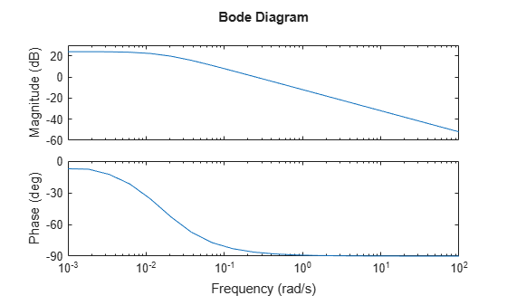
sys를 플로팅합니다.

bode(sys)

MATLAB figure

이산시간 MIMO 주파수 응답 데이터 모델

라이브 스크립트 열기

이 예제에서는 무작위로 생성된 응답 데이터와 주파수가 있다고 가정하겠습니다.

3×2×7 복소수 배열과, 0.01rad/s와 100rad/s 사이의 7개 점을 갖는 주파수 벡터를 생성합니다. 샘플 시간 Ts를 5초로 설정합니다.

rng(0)
r = randn(3,2,7)+1i*randn(3,2,7);
w = logspace(-2,2,7);
Ts = 5;

모델을 생성합니다.

sys = frd(r,w,Ts)

sys =

  From input 1 to:

    Frequency(rad/s)         output 1           output 2           output 3    
    ----------------         --------           --------           --------    
          0.0100         0.5377 + 0.3192i   1.8339 + 0.3129i  -2.2588 - 0.8649i
          0.0464        -0.4336 + 1.0933i   0.3426 + 1.1093i   3.5784 - 0.8637i
          0.2154         0.7254 - 0.0068i  -0.0631 + 1.5326i   0.7147 - 0.7697i
          1.0000         1.4090 - 1.0891i   1.4172 + 0.0326i   0.6715 + 0.5525i
          4.6416         0.4889 - 1.4916i   1.0347 - 0.7423i   0.7269 - 1.0616i
         21.5443         0.8884 - 0.1924i  -1.1471 + 0.8886i  -1.0689 - 0.7648i
        100.0000         0.3252 - 0.1774i  -0.7549 - 0.1961i   1.3703 + 1.4193i

  From input 2 to:

    Frequency(rad/s)         output 1           output 2           output 3    
    ----------------         --------           --------           --------    
          0.0100         0.8622 - 0.0301i   0.3188 - 0.1649i  -1.3077 + 0.6277i
          0.0464         2.7694 + 0.0774i  -1.3499 - 1.2141i   3.0349 - 1.1135i
          0.2154        -0.2050 + 0.3714i  -0.1241 - 0.2256i   1.4897 + 1.1174i
          1.0000        -1.2075 + 1.1006i   0.7172 + 1.5442i   1.6302 + 0.0859i
          4.6416        -0.3034 + 2.3505i   0.2939 - 0.6156i  -0.7873 + 0.7481i
         21.5443        -0.8095 - 1.4023i  -2.9443 - 1.4224i   1.4384 + 0.4882i
        100.0000        -1.7115 + 0.2916i  -0.1022 + 0.1978i  -0.2414 + 1.5877i
 
Sample time: 5 seconds
Discrete-time frequency response.
Model Properties

지정된 데이터로 2-입력, 3-출력 frd 모델이 생성됩니다.

상속된 속성이 있는 주파수 응답 데이터

라이브 스크립트 열기

이 예제에서는 전달 함수 모델에서 상속한 속성을 갖는 주파수 응답 데이터 모델을 만듭니다.

TimeUnit 속성이 'minutes'로, InputDelay 속성이 3으로 설정된 전달 함수 sys1을 만듭니다.

numerator1 = [2,0];
denominator1 = [1,8,0];
sys1 = tf(numerator1,denominator1,'TimeUnit','minutes','InputDelay',3)

sys1 =
 
                 2 s
  exp(-3*s) * ---------
              s^2 + 8 s
 
Continuous-time transfer function.
Model Properties

propValues1 = {sys1.TimeUnit,sys1.InputDelay}

propValues1=1×2 cell array
    {'minutes'}    {[3]}

sys1에서 상속한 속성으로 frd 모델을 만듭니다.

rng(0)
response = randn(1,1,7)+1i*randn(1,1,7);
w = logspace(-2,2,7);
sys2 = frd(response,w,sys1)

sys2 =
 
    Frequency(rad/minute)         Response    
    ---------------------         --------    
             0.0100           0.5377 + 0.3426i
             0.0464           1.8339 + 3.5784i
             0.2154          -2.2588 + 2.7694i
             1.0000           0.8622 - 1.3499i
             4.6416           0.3188 + 3.0349i
            21.5443          -1.3077 + 0.7254i
           100.0000          -0.4336 - 0.0631i
 
  Input delays (minutes): 3 
 
Continuous-time frequency response.
Model Properties

propValues2 = {sys2.TimeUnit,sys2.InputDelay}

propValues2=1×2 cell array
    {'minutes'}    {[3]}

frd 모델 sys2가 sys1과 동일한 속성을 가짐을 알 수 있습니다.

주파수 응답 데이터 모델의 상태 및 입력 이름 지정하기

라이브 스크립트 열기

이 예제에서는 물탱크 모델과 관련해 수집된 주파수 응답 데이터를 불러옵니다.

load wtankData.mat

이 모델에는 1개의 입력인 Voltage와 1개의 출력인 Water height가 있습니다.

입력 이름과 출력 이름을 지정하여 frd 모델을 만듭니다.

sys = frd(response,frequency,'InputName','Voltage','OutputName','Height');

주파수 응답을 플로팅합니다.

bode(sys)

MATLAB figure

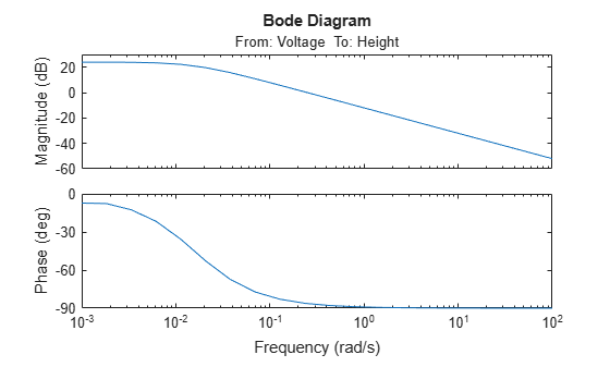
입력 이름과 출력 이름이 보드 플롯에 표시됩니다. 입력 이름과 출력 이름을 지정하면 MIMO 시스템의 응답 플롯을 처리할 때 유용할 수 있습니다.

상태공간 모델을 주파수 응답 데이터 모델로 변환하기

라이브 스크립트 열기

이 예제에서는 다음 상태공간 모델의 frd 모델을 계산합니다.

$A = [\begin{array}{c} - 2 & - 1 \\ 1 & - 2 \end{array}], B = [\begin{array}{c} 1 & 1 \\ 2 & - 1 \end{array}], C = [\begin{array}{c} 1 & 0 \end{array}], D = [\begin{array}{c} 0 & 1 \end{array}]$

상태공간 행렬을 사용하여 상태공간 모델을 만듭니다.

A = [-2 -1;1 -2];
B = [1 1;2 -1];
C = [1 0];
D = [0 1];
ltiSys = ss(A,B,C,D);

상태공간 모델 ltiSys를 0.01rad/s와 100rad/s 사이의 주파수에 대한 frd 모델로 변환합니다.

w = logspace(-2,2,50);
sys = frd(ltiSys,w);

주파수 응답을 비교합니다.

bode(ltiSys,'b',sys,'r--')

MATLAB figure

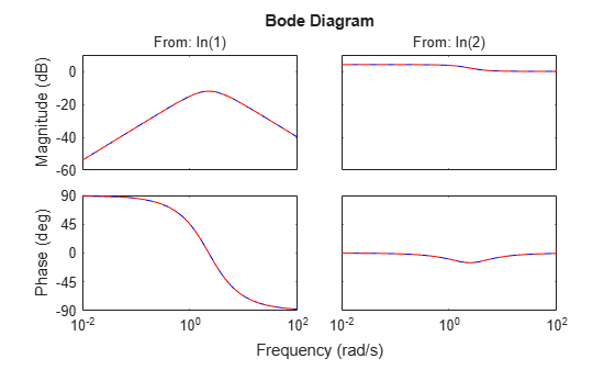
응답이 동일합니다.

주파수 응답 데이터 모델로 구성된 배열

라이브 스크립트 열기

frd 모델들로 구성된 배열을 만들려면 주파수 응답 데이터로 구성된 다차원 배열을 지정하면 됩니다.

예를 들어 응답 데이터를 크기가 [NY NU NF S1 ... Sn]인 숫자형 배열로 지정하면 함수는 frd 모델로 구성된 S1×...×Sn 배열을 반환합니다. 이러한 각 모델에는 NY개의 출력, NU개의 입력, NF개의 주파수 지점이 있습니다.

0.1rad/s와 10rad/s 사이의 10개 주파수 지점에서 1-출력, 2-입력 모델을 사용하여 무작위 응답 데이터로 구성된 2×3 배열을 생성합니다.

w = logspace(-1,1,10);
r = randn(1,2,10,2,3)+1i*randn(1,2,10,2,3);
sys = frd(r,w);

모델 배열에서 인덱스 (2,1)에 있는 모델을 추출합니다.

sys21 = sys(:,:,2,1)

sys21 =

  From input 1 to:

    Frequency(rad/s)         output 1    
    ----------------         --------    
          0.1000         0.6715 + 0.0229i
          0.1668         0.7172 - 1.7502i
          0.2783         0.4889 - 0.8314i
          0.4642         0.7269 - 1.1564i
          0.7743         0.2939 - 2.0026i
          1.2915         0.8884 + 0.5201i
          2.1544        -1.0689 - 0.0348i
          3.5938        -2.9443 + 1.0187i
          5.9948         0.3252 - 0.7145i
         10.0000         1.3703 - 0.2248i

  From input 2 to:

    Frequency(rad/s)         output 1    
    ----------------         --------    
          0.1000        -1.2075 - 0.2620i
          0.1668         1.6302 - 0.2857i
          0.2783         1.0347 - 0.9792i
          0.4642        -0.3034 - 0.5336i
          0.7743        -0.7873 + 0.9642i
          1.2915        -1.1471 - 0.0200i
          2.1544        -0.8095 - 0.7982i
          3.5938         1.4384 - 0.1332i
          5.9948        -0.7549 + 1.3514i
         10.0000        -1.7115 - 0.5890i
 
Continuous-time frequency response.
Model Properties

음수 주파수가 있는 주파수 응답 데이터 모델

라이브 스크립트 열기

frd 객체에 음수 주파수 값을 지정할 수 있습니다. 이 기능은 복소 계수를 갖는 모델의 주파수 응답 데이터를 캡처하고자 할 때 유용합니다.

양수 값과 음수 값이 모두 있는 주파수 벡터를 만듭니다.

w0 = sort([-logspace(-2,2,50) 0 logspace(-2,2,50)]);

복소 계수를 갖는 상태공간 모델을 만듭니다.

A = [-3.50,-1.25-0.25i;2,0];
B = [1;0];
C = [-0.75-0.5i,0.625-0.125i];
D = 0.5;
Gc = ss(A,B,C,D);

지정된 주파수에서 모델을 frd 모델로 변환합니다.

sys = frd(Gc,w0);

모델의 주파수 응답을 플로팅합니다.

bode(Gc,'b',sys,'r--')

MATLAB figure

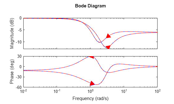
플롯 응답이 거의 일치합니다. 플롯에는 복소 계수를 갖는 모델에 대해 두 개의 분기가 표시되는데, 하나는 오른쪽을 가리키는 화살표가 있는 양수 주파수에 대한 것이고 다른 하나는 왼쪽을 가리키는 화살표가 있는 음수 주파수에 대한 것입니다. 두 분기에서 화살표는 주파수가 증가하는 방향을 나타냅니다.

버전 내역

R2006a 이전에 개발됨

참고 항목

get | set | ss | zpk | tf | frdata | genfrd | frdfun | bode | pidtune

frd

설명

생성

구문

설명

입력 인수

response — 주파수 응답 데이터 벡터 | 다차원 배열

frequency — 주파수 지점 벡터

ts — 샘플 시간 스칼라

ltiSys — 동적 시스템 동적 시스템 모델 | 모델 배열

속성

ResponseData — 주파수 응답 데이터 복소수로 구성된 다차원 배열

Frequency — 주파수 지점 벡터

FrequencyUnit — 주파수 벡터의 단위 'rad/TimeUnit' (디폴트 값) | 'cycles/TimeUnit' | 'rad/s' | 'Hz' | 'kHz' | 'MHz' | 'GHz' | 'rpm'

IODelay — 전송 지연 0 (디폴트 값) | 스칼라 | Ny×Nu 배열

InputDelay — 입력 지연 0 (디폴트 값) | 스칼라 | Nu×1 벡터

OutputDelay — 출력 지연 0 (디폴트 값) | 스칼라 | Ny×1 벡터

Ts — 샘플 시간 0 (디폴트 값) | 양의 스칼라 | -1

TimeUnit — 시간 변수 단위 'seconds' (디폴트 값) | 'nanoseconds' | 'microseconds' | 'milliseconds' | 'minutes' | 'hours' | 'days' | 'weeks' | 'months' | 'years' | ...

InputName — 입력 채널 이름 '' (디폴트 값) | 문자형 벡터 | 문자형 벡터로 구성된 셀형 배열

InputUnit — 입력 채널 단위 '' (디폴트 값) | 문자형 벡터 | 문자형 벡터로 구성된 셀형 배열

InputGroup — 입력 채널 그룹 구조체

OutputName — 출력 채널 이름 '' (디폴트 값) | 문자형 벡터 | 문자형 벡터로 구성된 셀형 배열

OutputUnit — 출력 채널 단위 '' (디폴트 값) | 문자형 벡터 | 문자형 벡터로 구성된 셀형 배열

OutputGroup — 출력 채널 그룹 구조체

Name — 시스템 이름 '' (디폴트 값) | 문자형 벡터

Notes — 사용자 지정 텍스트 {} (디폴트 값) | 문자형 벡터 | 문자형 벡터로 구성된 셀형 배열

UserData — 사용자 지정 데이터 [] (디폴트 값) | 모든 MATLAB® 데이터형

SamplingGrid — 모델 배열의 샘플링 그리드 구조체형 배열

객체 함수

주파수 응답 분석

모델 변환

모델 상호 연결

제어기 설계

예제

SISO 주파수 응답 데이터 모델

이산시간 MIMO 주파수 응답 데이터 모델

상속된 속성이 있는 주파수 응답 데이터

주파수 응답 데이터 모델의 상태 및 입력 이름 지정하기

상태공간 모델을 주파수 응답 데이터 모델로 변환하기

주파수 응답 데이터 모델로 구성된 배열

음수 주파수가 있는 주파수 응답 데이터 모델

버전 내역

참고 항목

도움말 항목

`response` — 주파수 응답 데이터
벡터 | 다차원 배열

`frequency` — 주파수 지점
벡터

`ts` — 샘플 시간
스칼라

`ltiSys` — 동적 시스템
동적 시스템 모델 | 모델 배열

`ResponseData` — 주파수 응답 데이터
복소수로 구성된 다차원 배열

`Frequency` — 주파수 지점
벡터

`FrequencyUnit` — 주파수 벡터의 단위
`'rad/TimeUnit'` (디폴트 값) | `'cycles/TimeUnit'` | `'rad/s'` | `'Hz'` | `'kHz'` | `'MHz'` | `'GHz'` | `'rpm'`

`IODelay` — 전송 지연
`0` (디폴트 값) | 스칼라 | `Ny`×`Nu` 배열

`InputDelay` — 입력 지연
`0` (디폴트 값) | 스칼라 | `Nu`×1 벡터

`OutputDelay` — 출력 지연
`0` (디폴트 값) | 스칼라 | `Ny`×1 벡터

`Ts` — 샘플 시간
`0` (디폴트 값) | 양의 스칼라 | `-1`

`TimeUnit` — 시간 변수 단위
`'seconds'` (디폴트 값) | `'nanoseconds'` | `'microseconds'` | `'milliseconds'` | `'minutes'` | `'hours'` | `'days'` | `'weeks'` | `'months'` | `'years'` | ...

`InputName` — 입력 채널 이름
`''` (디폴트 값) | 문자형 벡터 | 문자형 벡터로 구성된 셀형 배열

`InputUnit` — 입력 채널 단위
`''` (디폴트 값) | 문자형 벡터 | 문자형 벡터로 구성된 셀형 배열

`InputGroup` — 입력 채널 그룹
구조체

`OutputName` — 출력 채널 이름
`''` (디폴트 값) | 문자형 벡터 | 문자형 벡터로 구성된 셀형 배열

`OutputUnit` — 출력 채널 단위
`''` (디폴트 값) | 문자형 벡터 | 문자형 벡터로 구성된 셀형 배열

`OutputGroup` — 출력 채널 그룹
구조체

`Name` — 시스템 이름
`''` (디폴트 값) | 문자형 벡터

`Notes` — 사용자 지정 텍스트
`{}` (디폴트 값) | 문자형 벡터 | 문자형 벡터로 구성된 셀형 배열

`UserData` — 사용자 지정 데이터
`[]` (디폴트 값) | 모든 MATLAB^® 데이터형

`SamplingGrid` — 모델 배열의 샘플링 그리드
구조체형 배열