Compensator Design for a Set of Plant Models
This example shows how to design and analyze a controller for multiple plant models using Control System Designer.
Acquire a Set of Plant Models
For a typical feedback problem, the controller, C, is designed to satisfy some performance objective.

Typically, the dynamics of the plant, G, are not known exactly and can vary based on operating conditions. For example, the system dynamics can vary:
Due to manufacturing tolerances that are typically defined as a range about the nominal value. For example, resistors have a specified tolerance range, such as 5 ohms +/- 1%.
Operating conditions. For example, aircraft dynamics change based on altitude and speed.
When designing controllers for these types of systems, the performance objectives must be satisfied for all variations of the system.
You can model such systems as a set of LTI models stored in an LTI array. You can then use Control System Designer to design a controller for a nominal plant from the array and analyze the controller design for the entire set of plants.
The following list shows commands for creating an array of LTI models:
Control System Toolbox™:
Simulink® Control Design™:
Functions:
frestimate(Simulink Control Design),linearize(Simulink Control Design)Example: Reference Tracking of DC Motor with Parameter Variations (Simulink Control Design).
Robust Control Toolbox™:
System Identification Toolbox™:
Create LTI Array
In this example, the plant model is the second-order system:

where
 and
and  .
.
Construct an LTI array for the combinations of  and
and  .
.
wn = [1,1.5,2];
zeta = [.2,.5,.8];
ct = 1;
for ct1 = 1:length(wn)
    for ct2 = 1:length(zeta)
        zetai = zeta(ct2);
        wni = wn(ct1);
        G(1,1,ct) = tf(wni^2,[1,2*zetai*wni,wni^2]);
        ct = ct+1;
    end
end

size(G)
9x1 array of transfer functions.
Each model has 1 outputs and 1 inputs.
Open Control System Designer
Start the Control System Designer.
controlSystemDesigner(G)

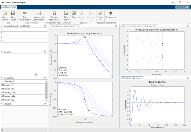
The app opens with Bode and root locus open-loop editors open along with a step response plot.
By default, the nominal model used for design is the first element in the LTI array.
The root locus editor displays the root locus for the nominal model and the closed-loop pole locations associated with the set of plants.
The Bode editor displays both the nominal model response and responses of the set of plants.
Using these editors, you can interactively tune the gain, poles, and zeros of the compensator, while simultaneously visualizing the effect on the set of plants.
Change the Nominal Model
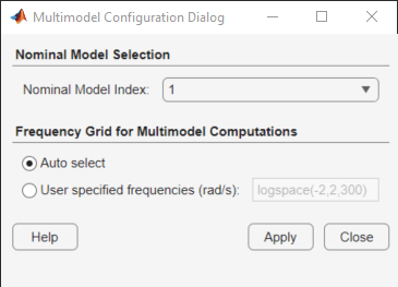
To change the nominal model, in the app, click Multimodel Configuration.

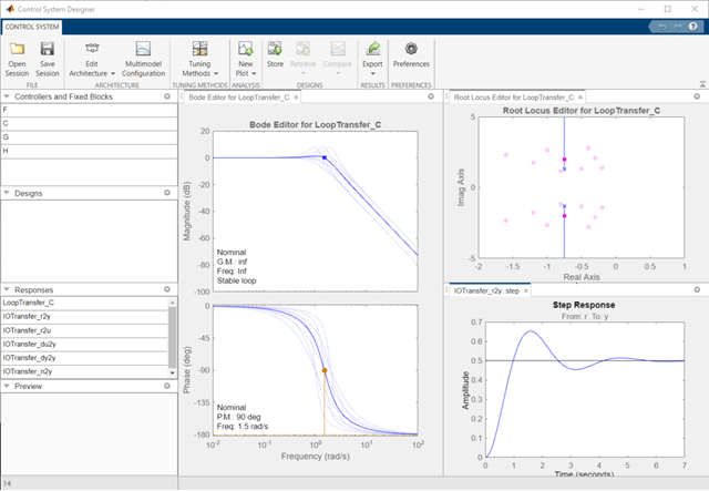
To select the fifth model in the array as the nominal model, in the Multimodel Configuration dialog box, set the Nominal Model Index to 5. The app response plots update automatically.

Options for Plotting Responses
The response plots always show the response of the nominal model. To view the other model responses, right-click the plot area and select:
Multimodel Display > Individual Responses to view the response for each model.
Multimodel Display > Bounds to view an envelope that encapsulates all of the responses.
