frestimate
Frequency response estimation of Simulink models
Syntax
Description
[___] = frestimate(___,
computes the frequency response using additional options. You can use this syntax with any
of the previous input and output argument combinations.options)
sysest = frestimate(data,freqs,units)
Examples
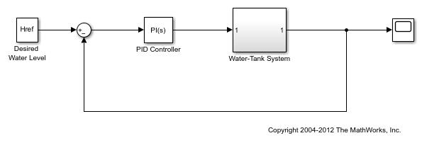
Estimate the open-loop response of the plant in the watertank model. Open the model.
model = 'watertank';
open_system(model)

To estimate the open-loop response of the plant, define a linearization I/O set that specifies this portion of the model with analysis points. Define an input analysis point at the controller output, and define an open-loop output point at the plant output.
io(1)=linio('watertank/PID Controller',1,'input');
io(2)=linio('watertank/Water-Tank System',1,'openoutput');
Find a steady-state operating point for the estimation. For this example, use a steady-state operating point derived from the model initial conditions.
watertank_spec = operspec(model);
opOpts = findopOptions('DisplayReport','off');
op = findop(model,watertank_spec,opOpts);
Create an input signal for estimation. For this example, use a sinestream signal, which sends a series of separate sinusoidal perturbations at the frequencies you specify.
input = frest.Sinestream('Frequency',logspace(-3,2,30));
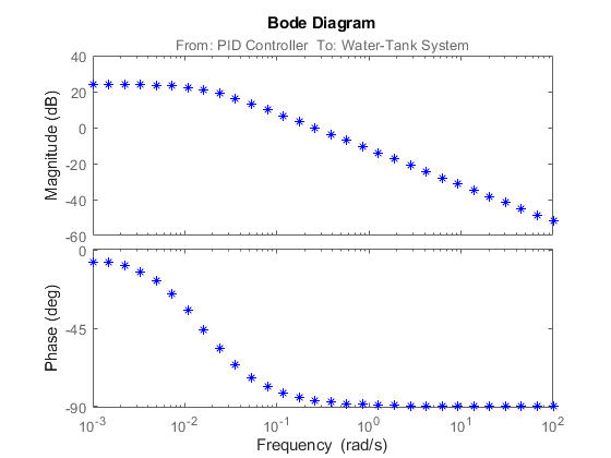
Estimate the frequency response of the specified portion of the model. The result is a frequency-response model containing responses at each of the frequencies specified in the sinestream signal.
sysest = frestimate(model,op,io,input);
size(sysest)
FRD model with 1 outputs, 1 inputs, and 30 frequency points.
Examine the measured frequency response.
bode(sysest,'*')
Linearize a Simulink model and use frequency-response estimation to validate the exact linearization results.
Open the watertank model.
model = 'watertank';
open_system(model);

Obtain a linearization of the open-loop response of the plant. To do so, define the linearization I/O points, and find a steady-state operating point near the model initial conditions. Then, linearize the model.
io(1)=linio('watertank/PID Controller',1,'input');
io(2)=linio('watertank/Water-Tank System',1,'openoutput');

watertank_spec = operspec(model);
opOpts = findopOptions('DisplayReport','off');
op = findop(model,watertank_spec,opOpts);

syslin = linearize(model,op,io);
To check the linearization, use the same analysis points and operating point to estimate the frequency response. For this example, use a sinestream input signal for the estimation.
input = frest.Sinestream('Frequency',logspace(-3,2,20));
sysest = frestimate(model,op,io,input);
Compare the exact linearization and the estimated response in the frequency domain using a Bode plot.
bode(syslin,'b-',sysest,'r*')
legend('Exact linearization','Estimation')

The Simulation Results Viewer lets you examine the results of frequency response estimation frequency by frequency. You open the viewer using the frest.simView command. To do so, store the simulation data using the simout output argument of frestimate.
Estimate the open-loop response of the plant in the watertank model. First, open the model.
model = 'watertank';
open_system(model)
Define a linearization I/O set that specifies the plant, and find a steady-state operating point for estimation.
io(1)=linio('watertank/PID Controller',1,'input');
io(2)=linio('watertank/Water-Tank System',1,'openoutput');

watertank_spec = operspec(model);
opOpts = findopOptions('DisplayReport','off');
op = findop(model,watertank_spec,opOpts);
Then, create an input signal for estimation, and estimate the frequency response of the specified portion of the model. Use the simout output argument to store the estimation data.
input = frest.Sinestream('Frequency',logspace(-3,2,10));
[sysest,simout] = frestimate(model,op,io,input);
Open the Simulation Results Viewer.
frest.simView(simout,input,sysest)
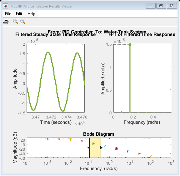
The viewer shows you the steady-state time response and the FFT of that response for all frequencies within the range you select on the Bode Diagram section of the viewer. These plots can help you identify when the response deviates from the expected response. For more information about using the Simulation Results Viewer, see Analyze Estimated Frequency Response.
If you have a linear model of the system you are estimating, you can use the model as a baseline response for comparison in the viewer. For instance, you can compare a model obtained by exact linearization to the estimated frequency response. Use the linearization I/O set and the operating point to compute an exact linearization of the watertank plant.
syslin = linearize(model,io,op);
Open the Simulation Results Viewer again, this time providing syslin as an input argument.
frest.simView(simout,input,sysest,syslin)
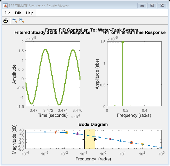
The Bode Diagram section of the viewer includes a line showing the exact response syslin. This view can be useful to identify particular frequencies where the estimated response deviates from the linearization.
Input Arguments
Output Arguments
Limitations
If you use
frestimatewith an output analysis point in a model reference, the Total number of instances allowed per top model configuration parameter of the referenced model must be 1.
Tips
For multiple-input multiple-output (MIMO) systems,
frestimateinjects the signal at each input channel separately to simulate the corresponding output signals. The estimation algorithm uses the inputs and the simulated outputs to compute the MIMO frequency response. If you want to inject different input signals at the linearization input points of a multiple-input system, treat your system as separate single-input systems. Perform independent frequency response estimations for each linearization input point usingfrestimate, and concatenate your frequency response results.
Algorithms
frestimate injects the input signal you specify (uest(t)) at the input analysis points. It simulates the model and collects the
response signal (yest(t)) at the output analysis points, as illustrated below for a sinestream
input.

In general, frestimate estimates the frequency response by computing
the ratio of the fast Fourier transforms output signal and the input signal:
For sinestream input signals, the function discards the data collected during the specified settling periods of the signal at each frequency. (See Sinestream Input Signals.) If the filtering option of the sinestream signal is active, the function then applies a bandpass filter to the remaining signal at the corresponding frequency and discards one more period to remove any remaining transient signals. The function uses the FFT of the resulting signal to compute Resp. The resulting
frdmodel contains all frequencies in the sinestream.
For chirp input signals, the function discards any frequencies in the ratio Resp that fall outside the frequency range specified for the chirp. The resulting
frdmodel contains all frequencies in the Fourier transform that fall within the chirp range.For other input signals, the resulting
frdcontains all the frequencies in the Fourier transform.
Extended Capabilities
Version History
Introduced in R2009b
See Also
frest.Sinestream | frest.Chirp | frest.Random | frest.simView | frestimateOptions | getSimulationTime