Derive Equations of Motion and Simulate Cart-Pole System

This example shows how to derive the equations of motion for the cart-pole system using Symbolic Math Toolbox™ and then simulate the cart-pole system using the ode45 solver. In the later sections of the example, you explore how to derive the equations in other forms that can be used to numerically simulate the system (and validate the results) using different tools, such as Simulink®, Simscape™ Multibody™, and Robotics System Toolbox™.

The equations of motion are crucial for modeling and simulating the system in dynamical systems and control theory. The stabilization of the cart-pole system, also known as the inverted pendulum, is one of the most widely used benchmark problems in control design and reinforcement learning [1].

Define Cart-Pole System

In the general cart-pole system, the pole is an object with a given mass and moment of inertia. The pole can be a rod with uniform density, or it can be a massless rod with another point mass attached to its end (an inverted pendulum). The cart-pole system includes a special case of an inverted pendulum with an attached object that does not move. Assume a fluid friction force, which also covers the special case where there is no friction. You can extend the assumed fluid friction force to a more complex friction model when needed.

This figure illustrates the cart-pole system discussed in this example.

To derive the equations of motion following Newton's second law, first define the symbolic variables. These parameters and variables describe the cart-pole system:

• t is the time.

• g is the gravitational acceleration.

• l is the distance from the pole-cart attachment to the pole's center of mass.

• I is the moment of inertia of the pole (with respect to the rotation axis at the center of mass).

• m is the mass of the pole.

• M is the mass of the cart.

• H and V are the horizontal and vertical forces on the pole, respectively. These forces form action and reaction pairs that act on both the pole and the cart. When acting on the pole, H is positive in the x-direction (right), while V is positive in the y-direction (up).

• F and dF are external forces acting on the cart and the center of mass of the pole, respectively.

• theta(t) is the angle that expresses the counterclockwise rotation of the pole with respect to the y-axis (so theta = 0 represents the pole standing upright on the cart).

• x(t) is the cart displacement with respect to its initial position along the x-direction.

In this example, the term $-\mathit{b}\frac{\mathrm{d}}{\mathrm{d}\mathit{t}}\mathit{x}\left(\mathit{t}\right)$ denotes the friction force on the cart due to the fluid or air surrounding it. If the cart slides on a surface (as opposed to, for example, being on wheels), then you need to use a more accurate model of kinetic friction force.

For an example that uses a different angle notation and includes a pole length of $$2l$$, see [2].

Derive Equations of Motion

The equations that represent the cart-pole system can be expressed in various forms, depending on the preferred notation, convention, and calculation sequence. However, it is known that the literature contains inaccuracies (for example, see [2] and [3]). This example uses an approach to deriving the equations that is similar to the first approach used in [3], but this section also explains how the equations can be written as in [2]. Later, you solve these equations to determine how the pole angle $$\theta (t)$$ and the cart displacement $$x(t)$$ evolve over time given some initial conditions.

Define Symbolic Variables

Define symbolic variables that represent the parameters and variables of the cart-pole system. Because the pole angle and cart displacement can change over time, define theta and x as functions of t.

syms t g l I m M H V F dF theta(t) x(t) b

Assume that some of the variables are positive. This simplification makes the representation of expressions involving these variables clearer and helps restrict the returned solutions to feasible domains.

assume([t g l m M b] > 0)

Also, assume that the other variables are real.

assume([I H V F dF],"real")

Derive Equations of Motion in Horizontal Direction

Based on Newton's second law, define an equation to express the horizontal forces acting on the cart. All the forces acting in the x-direction are on the left side of the equation, while the cart's mass multiplied by its acceleration is on the right side.

eq1 = F - H - b*diff(x,1) == M*diff(x,2)

eq1(t) = 
$$-b\hspace{0.17em}\frac{\partial }{\partial t}\mathrm{ }x\left(t\right)+F-H=M\hspace{0.17em}\frac{{\partial }^2}{\partial t^2}\mathrm{ }x\left(t\right)$$

Define another equation to express the horizontal forces acting on the pole. Here, the position of the pole's center of mass is expressed in terms of x and theta, and the second derivative of this position (its acceleration) is equal to the total force acting on the pole's end in the horizontal direction.

eq2 = H - dF == m*diff(x - l*sin(theta),2)

eq2(t) = 
$$H-\mathrm{dF}=m\hspace{0.17em}\left(\frac{{\partial }^2}{\partial t^2}\mathrm{ }x\left(t\right)+l\hspace{0.17em}\sin \left(\theta \left(t\right)\right)\hspace{0.17em}{\left(\frac{\partial }{\partial t}\mathrm{ }\theta \left(t\right)\right)}^2-l\hspace{0.17em}\cos \left(\theta \left(t\right)\right)\hspace{0.17em}\frac{{\partial }^2}{\partial t^2}\mathrm{ }\theta \left(t\right)\right)$$

To obtain an equation without the force H, combine eq1 and eq2 into an equation in which the term H is eliminated.

mainEq1 = eliminate([eq1 eq2],H) == 0

mainEq1(t) = 
$$F-\mathrm{dF}-m\hspace{0.17em}\frac{{\partial }^2}{\partial t^2}\mathrm{ }x\left(t\right)-b\hspace{0.17em}\frac{\partial }{\partial t}\mathrm{ }x\left(t\right)-M\hspace{0.17em}\frac{{\partial }^2}{\partial t^2}\mathrm{ }x\left(t\right)-l\hspace{0.17em}m\hspace{0.17em}\left(\sin \left(\theta \left(t\right)\right)\hspace{0.17em}{\left(\frac{\partial }{\partial t}\mathrm{ }\theta \left(t\right)\right)}^2-\cos \left(\theta \left(t\right)\right)\hspace{0.17em}\frac{{\partial }^2}{\partial t^2}\mathrm{ }\theta \left(t\right)\right)=0$$

The equation mainEq1 is the first main equation that links the second derivatives of x(t) and theta(t).

Derive Forces and Moments Acting on Pole

Next, define an equation to express the forces on the pole along the direction normal to the pole (the x'-direction in the figure). Here, the sum of the forces along x' in the figure is expressed on the left side of the equation. The right side represents the acceleration of the pole's center of mass along x', expressed in terms of x(t) and theta(t).

eq3 = -V*sin(theta) + m*g*sin(theta) - H*cos(theta) + dF*cos(theta) == m*l*diff(theta,2) - m*diff(x,2)*cos(theta)

eq3(t) = 
$$\mathrm{dF}\hspace{0.17em}\cos \left(\theta \left(t\right)\right)-V\hspace{0.17em}\sin \left(\theta \left(t\right)\right)-H\hspace{0.17em}\cos \left(\theta \left(t\right)\right)+g\hspace{0.17em}m\hspace{0.17em}\sin \left(\theta \left(t\right)\right)=l\hspace{0.17em}m\hspace{0.17em}\frac{{\partial }^2}{\partial t^2}\mathrm{ }\theta \left(t\right)-m\hspace{0.17em}\cos \left(\theta \left(t\right)\right)\hspace{0.17em}\frac{{\partial }^2}{\partial t^2}\mathrm{ }x\left(t\right)$$

Define another equation to express the pole's angular momentum around its center of mass as a function of its moment of inertia. Here, the sum of moments around the pole's center of mass is equal to its rotational acceleration multiplied by its moment of inertia with respect to its center of mass.

eq4 = V*l*sin(theta) + H*l*cos(theta) == I*diff(theta,t,2)

eq4(t) = 
$$H\hspace{0.17em}l\hspace{0.17em}\cos \left(\theta \left(t\right)\right)+V\hspace{0.17em}l\hspace{0.17em}\sin \left(\theta \left(t\right)\right)=\text{I}\hspace{0.17em}\frac{{\partial }^2}{\partial t^2}\mathrm{ }\theta \left(t\right)$$

To obtain an equation without the forces H and V, combine eq3 and eq4 into an equation in which both terms H and V are eliminated.

mainEq2 = eliminate([eq3 eq4],[H V]) == 0

mainEq2(t) = 
$$\mathrm{dF}\hspace{0.17em}l\hspace{0.17em}\cos \left(\theta \left(t\right)\right)-\text{I}\hspace{0.17em}\frac{{\partial }^2}{\partial t^2}\mathrm{ }\theta \left(t\right)-l^2\hspace{0.17em}m\hspace{0.17em}\frac{{\partial }^2}{\partial t^2}\mathrm{ }\theta \left(t\right)+l\hspace{0.17em}m\hspace{0.17em}\cos \left(\theta \left(t\right)\right)\hspace{0.17em}\frac{{\partial }^2}{\partial t^2}\mathrm{ }x\left(t\right)+g\hspace{0.17em}l\hspace{0.17em}m\hspace{0.17em}\sin \left(\theta \left(t\right)\right)=0$$

The equation mainEq2 is the second main equation that links the second derivatives of x(t) and theta(t).

Other Form of Inverted Pendulum Equation

If you set the second derivative of the cart position to zero in the second main equation, the resulting equation represents an inverted pendulum system (a pole attached to a cart that does not move).

eqInvPendulum = isolate(subs(mainEq2,diff(x,t,2),0),theta)

eqInvPendulum = 
$$\mathrm{dF}\hspace{0.17em}l\hspace{0.17em}\cos \left(\theta \left(t\right)\right)-\text{I}\hspace{0.17em}\frac{{\partial }^2}{\partial t^2}\mathrm{ }\theta \left(t\right)-l^2\hspace{0.17em}m\hspace{0.17em}\frac{{\partial }^2}{\partial t^2}\mathrm{ }\theta \left(t\right)+g\hspace{0.17em}l\hspace{0.17em}m\hspace{0.17em}\sin \left(\theta \left(t\right)\right)=0$$

A simple pendulum model (with a clockwise positive angle convention), where no force is applied to the pole ($$dF=0$$), is also derived in the example Simulate the Motion of the Periodic Swing of a Pendulum and implemented in Simscape Multibody in the example Model a Simple Pendulum (Simscape Multibody).

Convert Equations to State-Space Representation

The first and second main equations in mainEq1 and mainEq2 describe the dynamics of the cart-pole system. To obtain a state-space representation of the system dynamics, use odeToVectorField on the two main equations. The odeToVectorField function converts higher-order differential equations to a system of first-order differential equations in a vector of state variables $\mathit{Y}\left(\mathit{t}\right)={\left[\begin{array}{cccc}{\mathit{Y}}_1\left(\mathit{t}\right)& {\mathit{Y}}_2\left(\mathit{t}\right)& \cdots & {\mathit{Y}}_{\mathit{n}}\left(\mathit{t}\right)\end{array}\right]}^{\mathit{T}}$. By reducing the order of the equations, you can generate numeric functions that simulate the system in MATLAB and Simulink. You can then find the numeric solutions of the system by using the ode45 function.

[ssEqs,states] = odeToVectorField([mainEq1 mainEq2])

ssEqs = 
$$\begin{array}{l}\left(\begin{array}{c}{Y}_2\\ \frac{l\hspace{0.17em}\left(M\hspace{0.17em}\mathrm{dF}\hspace{0.17em}\cos \left(Y_1\right)+F\hspace{0.17em}m\hspace{0.17em}\cos \left(Y_1\right)+g\hspace{0.17em}{m}^2\hspace{0.17em}\sin \left(Y_1\right)-b\hspace{0.17em}m\hspace{0.17em}\cos \left(Y_1\right)\hspace{0.17em}{Y}_4+M\hspace{0.17em}g\hspace{0.17em}m\hspace{0.17em}\sin \left(Y_1\right)-l\hspace{0.17em}{m}^2\hspace{0.17em}\cos \left(Y_1\right)\hspace{0.17em}\sin \left(Y_1\right)\hspace{0.17em}{Y_2}^2\right)}{{\sigma }_1}\\ Y_4\\ -\frac{\text{I}\hspace{0.17em}\mathrm{dF}-F\hspace{0.17em}\text{I}+\text{I}\hspace{0.17em}b\hspace{0.17em}{Y}_4-F\hspace{0.17em}{l}^2\hspace{0.17em}m+\mathrm{dF}\hspace{0.17em}{l}^2\hspace{0.17em}m+l^3\hspace{0.17em}{m}^2\hspace{0.17em}\sin \left(Y_1\right)\hspace{0.17em}{Y_2}^2-\mathrm{dF}\hspace{0.17em}{l}^2\hspace{0.17em}m\hspace{0.17em}{\cos \left(Y_1\right)}^2+b\hspace{0.17em}{l}^2\hspace{0.17em}m\hspace{0.17em}{Y}_4-g\hspace{0.17em}{l}^2\hspace{0.17em}{m}^2\hspace{0.17em}\cos \left(Y_1\right)\hspace{0.17em}\sin \left(Y_1\right)+\text{I}\hspace{0.17em}l\hspace{0.17em}m\hspace{0.17em}\sin \left(Y_1\right)\hspace{0.17em}{Y_2}^2}{{\sigma }_1}\end{array}\right)\\ \\ \mathrm{where}\\ \\ \mathrm{ }{\sigma }_1=-l^2\hspace{0.17em}{m}^2\hspace{0.17em}{\cos \left(Y_1\right)}^2+l^2\hspace{0.17em}{m}^2+M\hspace{0.17em}{l}^2\hspace{0.17em}m+\text{I}\hspace{0.17em}m+\text{I}\hspace{0.17em}M\end{array}$$

states = 
$$\left(\begin{array}{c}\theta \\ \mathrm{Dtheta}\\ x\\ \mathrm{Dx}\end{array}\right)$$

The first output, ssEqs, shows the four first-order differential equations ${\left[\begin{array}{cccc}{\dot{\mathit{Y}}}_1\left(\mathit{t}\right)& {\dot{\mathit{Y}}}_2\left(\mathit{t}\right)& {\dot{\mathit{Y}}}_3\left(\mathit{t}\right)& {\dot{\mathit{Y}}}_4\left(\mathit{t}\right)\end{array}\right]}^{\mathit{T}}$ in terms of four state variables ${\left[\begin{array}{cccc}{\mathit{Y}}_1\left(\mathit{t}\right)& {\mathit{Y}}_2\left(\mathit{t}\right)& {\mathit{Y}}_3\left(\mathit{t}\right)& {\mathit{Y}}_4\left(\mathit{t}\right)\end{array}\right]}^{\mathit{T}}$. The second output, states, indicates the relationship between the state variables and the degrees of freedom, theta(t) and x(t), which can expressed as

$${\mathit{Y}}_1\left(\mathit{t}\right)=\theta \left(\mathit{t}\right),{\mathit{Y}}_2\left(\mathit{t}\right)=\frac{\partial }{\partial \mathit{t}}\theta \left(\mathit{t}\right)=\dot{\theta }\left(\mathit{t}\right),{\mathit{Y}}_3\left(\mathit{t}\right)=\mathit{x}\left(\mathit{t}\right),{\mathit{Y}}_4\left(\mathit{t}\right)=\frac{\partial }{\partial \mathit{t}}\mathit{x}\left(\mathit{t}\right)=\dot{\mathit{x}}\left(\mathit{t}\right).$$

For more information on state-space representations of linear systems within system identification and control settings, see What Are State-Space Models? (System Identification Toolbox) and State-Space Realizations (Control System Toolbox), respectively.

Next, convert the symbolic form of the system of differential equations to a MATLAB® function by using matlabFunction. Specify the Vars name-value argument as a string array that represent all quantities in the equations. The generated anonymous function computes the time derivative of the vector Y(t) given the current value of time t for specified constant values of other known parameters (for more information, see Anonymous Functions). Although the generated function does not explicitly use t (the time derivatives of the state variables are not explicitly time dependent), you can still specify t as an argument for a more general case.

Ydot = matlabFunction(ssEqs,Vars=["t","Y","F","dF","I","M","b","g","l","m"]);

You can use this generated function to evaluate the time derivative of the state variables given some initial conditions and a set of parameters. For example, set the initial values of all state variables to zero, the forces on the cart and pole to 0.2 N, the moment of inertia to zero, the cart mass to 1 kg, the friction coefficient to zero, the gravitational acceleration to 9.81 m/s², the length from the pole-cart attachment to the pole's center of mass to 0.5 m, and the pole mass to 0.1 kg.

Ydot_init = Ydot(0,[0 0 0 0]',0.2,0.2,0,1,0,9.81,0.5,0.1)

Ydot_init = 4×1

         0
    4.4000
         0
    0.2000

Find Open-Loop Solution of Cart-Pole System

In this section, you express the open-loop solution of the cart-pole system in MATLAB, Simulink, and Robotics System Toolbox and find the solution by using the ode45 solver.

An open-loop solution to the system of differential equations is a solution in which the external forces acting on the system, F and dF, are independent of the state variables (without any feedback from the state variables of the system). In other words, the external forces do not depend on the state of the system. The forces follow a predefined model without the need to adjust based on actual output or conditions of the system.

Find Open-Loop Solution in MATLAB

To simulate the system in open loop from 0 to 10 seconds, you can use ode45. Because the first argument of ode45 must be a function that accepts exactly two input arguments, the time and the state vectors (t and Y), specify another function that takes exactly these two input arguments with defined parameters. Define the other function as Ydot_eval that evaluates Ydot using specified constant values for all other parameters outside t and Y. For example, specify the values of F as 0.2, dF as 0, I as 0.1/12, M as 1, b as 0, g as 9.81, l as 0.5, and m as 0.1.

Fval = 0.2;
dFval = 0;
Ival = 0.1/12;
Mval = 1;
bval = 0;
gval = 9.81;
lval = 0.5;
mval = 0.1;
Ydot_eval = @(t,Y) Ydot(t,Y,Fval,dFval,Ival,Mval,bval,gval,lval,mval)

Ydot_eval = function_handle with value:
    @(t,Y)Ydot(t,Y,Fval,dFval,Ival,Mval,bval,gval,lval,mval)

Define an initial condition where all four state variables are zero. Find the open-loop solution using ode45. Because the system starts from an unstable equilibrium, to minimize numerical errors, pass an odeset options structure specifying low relative and absolute error tolerances.

Y_init = zeros(4,1);
Ysol = ode45(Ydot_eval,[0 10],Y_init,odeset(RelTol=1e-12,AbsTol=1e-12));

Plot the solution for the second state variable, which is the pole's angular speed $$\underset{}{\overset{\dot{}}{\theta }}(t)$$, as a function of time.

fig1 = figure;
plot(Ysol.x,Ysol.y(2,:))
xlabel("Time (s)")
ylabel("d\theta/dt")
title("Open-Loop Solution of Cart-Pole System")

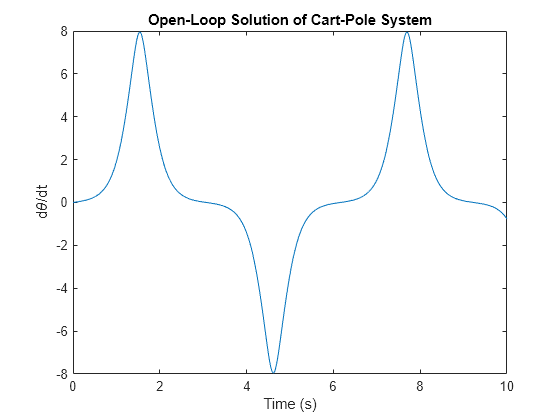
Note that to find analytical solutions of linear ordinary differential equations that can be expressed in closed-form mathematical expressions, you can use the dsolve function. For an example, see Simulate the Motion of the Periodic Swing of a Pendulum. However, for nonlinear ordinary differential equations, analytical solutions often do not exist or they exist in formulas that are too long to allow for useful insights into how the solutions interact with all quantities.

Find Open-Loop Solution in Simulink

Simulink provides a block diagram environment for multidomain simulation that is especially useful for designing and simulating systems containing several interacting components that can represented by both continuous and discrete-time systems (or systems using different sampling rates). There are several ways to express the cart-pole system in Simulink, which will be discussed in the next sections.

One way to build a Simulink model that express the cart-pole system is to use the state-space equations ssEqs obtained previously. First, create a new empty model named cp_sim.

new_system("cp_sim")

Open the model.

open_system("cp_sim")

Use the matlabFunctionBlock function to generate a Simulink block named YdotBlock that calculates the time derivatives of the state variables, with input ports for the current time, the current state variables, and the specified values of the other system parameters. Specify the name and path of the generated block in the cp_sim model as the first argument of matlabFunctionBlock, the state-space equations as the second argument, and the block input quantities as the third argument. Even if the time derivatives of the state variables do not explicitly depend on time, for this example, include the time variable as a block input.

matlabFunctionBlock("cp_sim/YdotBlock",ssEqs,Vars=["t","Y","F","dF","I","M","b","g","l","m"]);

Next, manually add blocks that specify the current time, current state variables, and the values of the other system parameters as inputs to YdotBlock. Create the additional Clock block, Integrator block, and Constant blocks. Add a To Workspace block that collects the values of the state variables into the workspace variable out.Ysol. Connect the blocks as shown in the following figure. For this example, the model with the generated block and additional blocks is attached in the file cp_sim.slx.

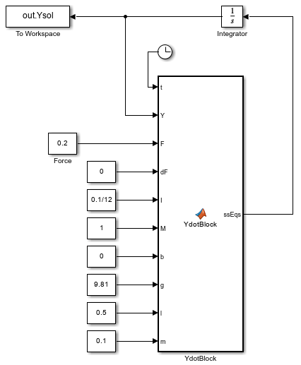
The Integrator block, with the label $$\frac{1}{s}$$, takes the time derivative of the state vector and returns the current value of the state vector Y. The Integrator block uses an integration algorithm that can be configured in the Solver pane of the Configuration Parameters dialog box. To open the Configuration Parameters dialog box, click Model Settings on the Modeling tab. Here, the initial condition of the Integrator block is set to zero.

As discussed in the previous section, because this system starts from an unstable equilibrium, select the ode45 integration and specify low relative and absolute error tolerances to minimize numerical errors.

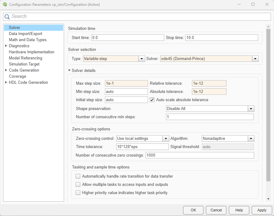
Finally, simulate the cart-pole system and find the open-loop solution. You can then plot the solution in out.Ysol to verify that the results are identical to those obtained using ode45 in previous subsection.

Find Open-Loop Solution in Robotics System Toolbox

You can also represent and simulate the cart-pole system in Robotics System Toolbox.

First, create a tree-structured object by using rigidBodyTree (Robotics System Toolbox) and define the gravity.

rbt = rigidBodyTree(DataFormat="column");
rbt.Gravity = [0 -9.81 0];

Create a rigid body object for the cart by using rigidBody (Robotics System Toolbox) and define the inertial properties of the cart.

cart = rigidBody("cart");
cart.Mass = 1;
cart.Inertia = zeros(1,6);

Create a prismatic joint by using rigidBodyJoint (Robotics System Toolbox). This joint attaches the cart to the rigid body tree and allows it to move along the x-axis.

cart.Joint = rigidBodyJoint("j1","prismatic");
cart.Joint.JointAxis = [1 0 0];

Add the cart to the rigid body tree by using addBody (Robotics System Toolbox).

addBody(rbt,cart,rbt.BaseName);

Next, create a rigid body object for the pole and its inertial properties. To follow the base coordinate system of the rigid body tree model, the angular position of the pole (counterclockwise positive) is zero when the pole is in the horizontal position. The pole length spans the x-axis with its center of mass at 0.5 m. In this coordinate system, the moment of inertia of the pole along the y- and z-axes, with respect to the attachment point, is $\frac{1}{3}{\mathit{m}\cdot \left(2\mathit{l}\right)}^2=\frac{1}{3}0.1\cdot 1^2=\frac{1}{30}$.

rod = rigidBody("rod");
rod.Mass = 0.1;
rod.CenterOfMass = [0.5 0 0];
rod.Inertia = [0 1/30 1/30 0 0 0];

Create a revolute joint that attaches the pole to the cart. Specify the fixed transformation for this joint that rotates the pole's coordinate system by $$\pi /2$$ along the z-axis. This rotation brings the pole's coordinate system in line with the one shown at the beginning of this example.

rod.Joint = rigidBodyJoint("j2","revolute");
setFixedTransform(rod.Joint,eul2tform([pi/2 0 0]));

Add the pole to the rigid body tree.

addBody(rbt,rod,cart.Name);

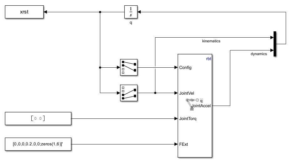
Next, define the helper function fd that takes a vector q containing the four state variables (cart's position, pole's position, cart's velocity, and pole's angular velocity) and returns the vector dqdt containing the time derivatives of q. This function uses the forwardDynamics (Robotics System Toolbox) function to calculate the joint accelerations, given the rigid body tree object, the joint positions and velocities, and the external force. You use this helper function as the first argument of the ode45 function when solving for the dynamics of the system. Specify the external force F acting on the cart to be 0.2 N. To simulate the system in a closed loop, you can set F as a function of q.

function dqdt = fd(~,q,rbt)

% Extract joint position, velocity and forces.
jointpos = q(1:2);
jointvel = q(3:4);
jointtau = zeros(2,1);

% Define external forces.
fext = externalForce(rbt,"cart",[0 0 0 0.2 0 0]);

% Calculate double derivatives of x and theta.
qdd = forwardDynamics(rbt,jointpos,jointvel,jointtau,fext);

% Assemble state vector.
dqdt = [jointvel; qdd];

end

Use ode45 to simulate the system in open loop from 0 to 10 seconds, starting with an initial condition where all four state variables are zero. Because the first argument of ode45 must be a function with exactly two input arguments (time and the state vector), you cannot call fd directly when using ode45. Instead, define an anonymous function that calls fd with a specified rigid body tree rbt. Because the system starts from an unstable equilibrium, to minimize numerical errors, pass an odeset options structure specifying low relative and absolute error tolerances.

Qsol = ode45(@(t,q) fd(t,q,rbt),[0 10],zeros(1,4),odeset(MaxStep=0.1,AbsTol=1e-12,RelTol=1e-12));

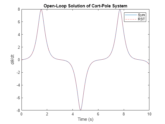
Plot the simulation results on the figure from the Find Open-Loop Solution in MATLAB section. The solution for the angular velocity perfectly overlaps with the solution of the equations of motion derived using Symbolic Math Toolbox.

figure(fig1)
hold on
plot(Qsol.x,Qsol.y(4,:),"r:")
legend("Sym","RST")
hold off

As an alternative to ode45, you can also use the Forward Dynamics (Robotics System Toolbox) block to simulate the system in Simulink. This block uses the rigid body tree rbt as an input parameter, takes the current positions and velocities of the joint as inputs, takes the external torques and forces acting on the bodies as inputs, and returns the joint accelerations as the output. You can also simulate a closed-loop system by replacing the constant force with a force that is a function of the joint positions and velocities.

Find Closed-Loop Solution of Cart-Pole System

A closed-loop control system uses feedback to control the states or outputs of a dynamical system. The closed-loop solution exists when the external forces acting on the system are functions of the state variables, which include the linear and angular positions and their velocities. In this section, you use Simulink Control Design™ to linearize the cart-pole system around the analysis points and use Control System Toolbox™ to compute the optimal gain matrix. Then you rewrite the external force as functions of the state variables and find the closed-loop solution of the cart-pole system by using ode45.

Find Operating Points, Linearization, and Control Synthesis

If your dynamical system is represented by a Simulink model, you can use an array of tools to find specific operating points, linearize the system around these points, and design controllers that stabilize and guide the systems from one operating point to another. For more information, see About Operating Points (Simulink Control Design), findopOptions (Simulink Control Design), and trim (Simulink).

In the cp_sim model, set the force acting on the cart to zero.

set_param("cp_sim/Force","Value","0")

Define input and output points of the system for linearization. Create linear analysis points using linio (Simulink Control Design). Add an input corresponding to the force on the cart (the output of the Force block), and add an output corresponding to the current state vector (the output of the integrator block).

io(1) = linio("cp_sim/Force",1,"input");
io(2) = linio("cp_sim/Integrator",1,"output");

Use linearize (Simulink Control Design) to linearize the model from the selected input to the selected output around the analysis points defined by the initial values of the state variables, which are zero, and the input force, which is also zero.

lsys = linearize("cp_sim",io);

Display the state and input matrices.

lsys.A

ans = 4×4

         0    1.0000         0         0
   15.7917         0         0         0
         0         0         0    1.0000
    0.7178         0         0         0

lsys.B

ans = 4×1

         0
    1.4634
         0
    0.9756

For more information about linearizing dynamical systems, see Linearize Nonlinear Models (Simulink Control Design).

Calculate the eigenvalues of the state matrix.

eig(lsys.A)

ans = 4×1

         0
         0
    3.9739
   -3.9739

One of these eigenvalues is positive, which means that the linearized system is unstable. In other words, the cart-pole system is unstable around the selected operating point. When the pole is in the upright position, a small disturbance leads to the pole falling and the cart moving.

Find the optimal gain matrix or state feedback by using the lqr (Control System Toolbox) function. Specify the weight matrices for the states and inputs as the third and fourth input arguments of lqr, respectively.

K = lqr(lsys.A,lsys.B,diag([10,10,0.1,1]),0.1)

K = 1×4

   49.0837   15.8752   -1.0000   -4.2198

For more information about designing control for linear and nonlinear systems, see Control System Modeling with Model Objects (Control System Toolbox), What Is Model Predictive Control? (Model Predictive Control Toolbox), and Reinforcement Learning for Control Systems Applications (Reinforcement Learning Toolbox).

Find Closed-Loop Solution Using ode45

Now, find the closed-loop solution of the cart-pole system using ode45, incorporating the optimal gain matrix you previously calculated. Replace the force F with the scalar inner product between -K and the vector containing the four state variables in the two main equations. Then compute the state-space equations for the closed-loop system.

[ssEqsCl,statesCl] = odeToVectorField(subs([mainEq1; mainEq2],F, ...
  -K*[theta(t); diff(theta(t),t); x(t); diff(x(t),t)])); 

Display the state variables of the system in terms of the degrees of freedom, theta(t) and x(t).

statesCl

statesCl = 
$$\left(\begin{array}{c}x\\ \mathrm{Dx}\\ \theta \\ \mathrm{Dtheta}\end{array}\right)$$

Note that the order of the returned state variables is different from the order of state variables returned in the open-loop state-space equations.

Substitute the value of dF with 0 and other constant parameters in the state-space equations with the values defined previously.

ssEqsCl = subs(ssEqsCl,[dF,I,M,b,g,l,m],[0,Ival,Mval,bval,gval,lval,mval]);

Generate a MATLAB function that calculates the time-derivative of the state vector given the current time and state vector.

YdotCl = matlabFunction(ssEqsCl,vars=["t","Y"]);

Simulate the system for 15 seconds, starting from an initial theta value of 0.1.

YsolCl = ode45(@(t,Y) YdotCl(t,Y),[0 15],[0 0 0.1 0]);

Plot the closed-loop solution of the system, which is the time evolution of the state variables.

figure;
plot(YsolCl.x,YsolCl.y)
xlabel("Time (s)")
ylabel("State Vector")
title("Closed-Loop Solution of Cart-Pole System")
legend("x","dx/dt","\theta","d\theta/dt",Location="east")

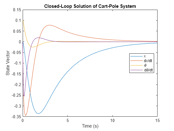
Even though the initial pole angle is 0.1, the force applied to the cart is able to bring the system back into the upright position. In other words, the upright position for this closed-loop system is a stable equilibrium.

Convert Equations of Motion to Mass-Matrix Representation

In addition to the state-space representation, you can rewrite the two main equations that describe the dynamics of the cart-pole system using mass-matrix representation. In this representation, you isolate the second-order derivatives of the horizontal and the angular positions of the system on the left side of the equations of motion. In other words, you express the cart-pole system equations in a form similar to Newton's second law, which is $$M(q)\underset{}{\overset{¨}{q}}=F(q,\underset{}{\overset{\dot{}}{q}},t)$$, where $$q(t)=[x(t),\theta (t){]}^T$$ and $$M(q)$$ is a 2-by-2 mass matrix that is a function of $$q$$.

For a system of ordinary differential equations, Symbolic Math Toolbox provides the massMatrixForm function to convert the system to first-order differential algebraic equations (DAEs). However, this function converts the system into the form $$M(t,y)\underset{}{\overset{\dot{}}{y}}=F(t,y)$$. For this reason, to use massMatrixForm to convert the system into the form with second-order derivatives, define the symbolic functions Dx(t) and Dtheta(t) to represent $$\underset{}{\overset{\dot{}}{x}}(t)$$ and $$\underset{}{\overset{\dot{}}{\theta }}(t)$$, respectively. Replace the first derivative terms in the main equations with these symbolic functions.

syms Dx(t) Dtheta(t)
mainEq1subs = subs(mainEq1,[diff(x,t) diff(theta,t)],[Dx Dtheta]);
mainEq2subs = subs(mainEq2,[diff(x,t) diff(theta,t)],[Dx Dtheta]);

Convert the main equations into the form $$M(t,y)\underset{}{\overset{\dot{}}{y}}=F(t,y)$$, where $$y(t)=[\underset{}{\overset{\dot{}}{x}}(t),\underset{}{\overset{\dot{}}{\theta }}(t){]}^T$$. Without loss of generality, consider the negative of the two main equations and convert them to the mass-matrix representation.

[matrixM,matrixF] = massMatrixForm([-mainEq1subs -mainEq2subs],[Dx Dtheta])

matrixM = 
$$\left(\begin{array}{cc}M+m& -l\hspace{0.17em}m\hspace{0.17em}\cos \left(\theta \left(t\right)\right)\\ -l\hspace{0.17em}m\hspace{0.17em}\cos \left(\theta \left(t\right)\right)& m\hspace{0.17em}{l}^2+\text{I}\end{array}\right)$$

matrixF = 
$$\left(\begin{array}{c}-l\hspace{0.17em}m\hspace{0.17em}\sin \left(\theta \left(t\right)\right)\hspace{0.17em}{\mathrm{Dtheta}\left(t\right)}^2+F-\mathrm{dF}-b\hspace{0.17em}\mathrm{Dx}\left(t\right)\\ \mathrm{dF}\hspace{0.17em}l\hspace{0.17em}\cos \left(\theta \left(t\right)\right)+g\hspace{0.17em}l\hspace{0.17em}m\hspace{0.17em}\sin \left(\theta \left(t\right)\right)\end{array}\right)$$

Next, in the matrix $$F$$, replace the symbolic functions Dx(t) and Dtheta(t) with the first-order derivatives that they represent, namely, $$\underset{}{\overset{\dot{}}{x}}(t)$$ and $$\underset{}{\overset{\dot{}}{\theta }}(t)$$.

matrixF = subs(matrixF,[Dx Dtheta],[diff(x,t) diff(theta,t)])

matrixF = 
$$\left(\begin{array}{c}-l\hspace{0.17em}m\hspace{0.17em}\sin \left(\theta \left(t\right)\right)\hspace{0.17em}{\left(\frac{\partial }{\partial t}\mathrm{ }\theta \left(t\right)\right)}^2-b\hspace{0.17em}\frac{\partial }{\partial t}\mathrm{ }x\left(t\right)+F-\mathrm{dF}\\ \mathrm{dF}\hspace{0.17em}l\hspace{0.17em}\cos \left(\theta \left(t\right)\right)+g\hspace{0.17em}l\hspace{0.17em}m\hspace{0.17em}\sin \left(\theta \left(t\right)\right)\end{array}\right)$$

Using the mass-matrix representation, you can derive the equations for the linear acceleration of the two degrees of freedom as functions of their velocities, positions, and all other parameters. In other words, you can represent the equations of motion as $$\underset{}{\overset{¨}{q}}=M^{-1}(q)F(q,\underset{}{\overset{\dot{}}{q}},t)$$.

D2q_eqn = [diff(x(t),t,2); diff(theta(t),t,2)] == inv(matrixM)*matrixF

D2q_eqn = 
$$\begin{array}{l}\left(\begin{array}{c}\frac{{\partial }^2}{\partial t^2}\mathrm{ }x\left(t\right)=\frac{l\hspace{0.17em}m\hspace{0.17em}\cos \left(\theta \left(t\right)\right)\hspace{0.17em}{\sigma }_3}{{\sigma }_1}-\frac{\left(m\hspace{0.17em}{l}^2+\text{I}\right)\hspace{0.17em}{\sigma }_2}{{\sigma }_1}\\ \frac{{\partial }^2}{\partial t^2}\mathrm{ }\theta \left(t\right)=\frac{\left(M+m\right)\hspace{0.17em}{\sigma }_3}{{\sigma }_1}-\frac{l\hspace{0.17em}m\hspace{0.17em}\cos \left(\theta \left(t\right)\right)\hspace{0.17em}{\sigma }_2}{{\sigma }_1}\end{array}\right)\\ \\ \mathrm{where}\\ \\ \mathrm{ }{\sigma }_1=-l^2\hspace{0.17em}{m}^2\hspace{0.17em}{\cos \left(\theta \left(t\right)\right)}^2+l^2\hspace{0.17em}{m}^2+M\hspace{0.17em}{l}^2\hspace{0.17em}m+\text{I}\hspace{0.17em}m+\text{I}\hspace{0.17em}M\\ \\ \mathrm{ }{\sigma }_2=l\hspace{0.17em}m\hspace{0.17em}\sin \left(\theta \left(t\right)\right)\hspace{0.17em}{\left(\frac{\partial }{\partial t}\mathrm{ }\theta \left(t\right)\right)}^2+b\hspace{0.17em}\frac{\partial }{\partial t}\mathrm{ }x\left(t\right)-F+\mathrm{dF}\\ \\ \mathrm{ }{\sigma }_3=\mathrm{dF}\hspace{0.17em}l\hspace{0.17em}\cos \left(\theta \left(t\right)\right)+g\hspace{0.17em}l\hspace{0.17em}m\hspace{0.17em}\sin \left(\theta \left(t\right)\right)\end{array}$$

Define the variable q_acc to represent the linear acceleration, which is equal to the right side of the previous equation. You can use this variable to formulate the time evolution of the two degrees of freedom across other engineering applications.

q_acc = rhs(D2q_eqn);

Cart-Pole System in Other Examples

Examples of Cart-Pole System in Model Predictive Control Toolbox

Several examples in the Model Predictive Control Toolbox™ documentation show how to control a cart-pole system using linear and nonlinear model predictive controls. For more details, see MPC Control of an Inverted Pendulum on a Cart (Model Predictive Control Toolbox), Explicit MPC Control of an Inverted Pendulum on a Cart (Model Predictive Control Toolbox), Time-Varying MPC Control of an Inverted Pendulum on a Cart (Model Predictive Control Toolbox), and Gain-Scheduled MPC Control of Inverted Pendulum on Cart (Model Predictive Control Toolbox).

For these examples, the pole is represented by a point mass with a moment of inertia of zero with respect to the center of mass. The quantities involved in the system equations are represented with Simulink blocks. The two inputs are the external forces acting on the pole and cart, and the four outputs are the cart position and velocity, as well as the pole's angular position and velocity.

This Simulink model represents the system.

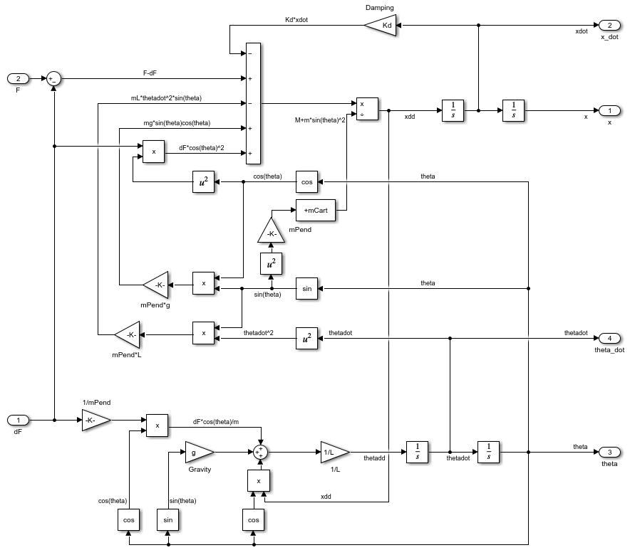
Derive the acceleration of the cart, indicated by the xdd label in the model, by using the first equation of the mass-matrix representation defined previously. The blocks leading up to xdd represent the terms on the right side of this equation.

xdd_eqn = diff(x(t),t,2) == simplify(subs(q_acc(1),I,0),Steps=100)

xdd_eqn = 
$$\frac{{\partial }^2}{\partial t^2}\mathrm{ }x\left(t\right)=\frac{F-b\hspace{0.17em}\frac{\partial }{\partial t}\mathrm{ }x\left(t\right)+\frac{M\hspace{0.17em}\mathrm{dF}}{m}+\frac{g\hspace{0.17em}m\hspace{0.17em}\sin \left(2\hspace{0.17em}\theta \left(t\right)\right)}{2}-l\hspace{0.17em}m\hspace{0.17em}\sin \left(\theta \left(t\right)\right)\hspace{0.17em}{\left(\frac{\partial }{\partial t}\mathrm{ }\theta \left(t\right)\right)}^2}{m\hspace{0.17em}{\sin \left(\theta \left(t\right)\right)}^2+M}-\frac{\mathrm{dF}}{m}$$

Derive the angular acceleration of the pole, indicated by the thetadd label in the model, by using the second main equation defined at the beginning of this example.

thetadd_eqn = subs(isolate(mainEq2,diff(theta(t),t,2)),I,0)

thetadd_eqn = 
$$\frac{{\partial }^2}{\partial t^2}\mathrm{ }\theta \left(t\right)=\frac{l\hspace{0.17em}m\hspace{0.17em}\cos \left(\theta \left(t\right)\right)\hspace{0.17em}\frac{{\partial }^2}{\partial t^2}\mathrm{ }x\left(t\right)+\mathrm{dF}\hspace{0.17em}l\hspace{0.17em}\cos \left(\theta \left(t\right)\right)+g\hspace{0.17em}l\hspace{0.17em}m\hspace{0.17em}\sin \left(\theta \left(t\right)\right)}{l^2\hspace{0.17em}m}$$

In other examples, such as Swing-Up Control of Pendulum Using Nonlinear Model Predictive Control (Model Predictive Control Toolbox) and Swing-Up Control of a Pendulum on a Cart using Multistage Nonlinear MPC with Nonlinear Grey-Box Model (Model Predictive Control Toolbox), the nonlinear plant model is defined in a MATLAB file in which the force on the pole is not considered (dF = 0), the horizontal axis is indicated as $$z$$ instead of $$x$$, and the friction coefficient is indicated as $$Kd$$ instead of $$b$$. Derive the acceleration of the cart from the previous equation xdd_eqn by setting dF to zero and replacing the variables $$x$$ and $$b$$ with $$z$$ and $$Kd$$, respectively.

syms z(t) Kd
xdd_eqn = subs(xdd_eqn,[dF x(t) b],[0 z(t) Kd])

xdd_eqn = 
$$\frac{{\partial }^2}{\partial t^2}\mathrm{ }z\left(t\right)=\frac{-l\hspace{0.17em}m\hspace{0.17em}\sin \left(\theta \left(t\right)\right)\hspace{0.17em}{\left(\frac{\partial }{\partial t}\mathrm{ }\theta \left(t\right)\right)}^2-\mathrm{Kd}\hspace{0.17em}\frac{\partial }{\partial t}\mathrm{ }z\left(t\right)+F+\frac{g\hspace{0.17em}m\hspace{0.17em}\sin \left(2\hspace{0.17em}\theta \left(t\right)\right)}{2}}{m\hspace{0.17em}{\sin \left(\theta \left(t\right)\right)}^2+M}$$

Derive the angular acceleration of the pole by using the second mass-matrix equation defined previously.

thetadd_eqn = diff(theta(t),t,2) == subs(q_acc(2),[I dF x(t) b],[0 0 z(t) Kd]);
thetadd_eqn = collect(isolate(thetadd_eqn,g*sin(theta(t))),diff(theta(t),t,2))

thetadd_eqn = 
$$g\hspace{0.17em}\sin \left(\theta \left(t\right)\right)=\frac{-l\hspace{0.17em}m\hspace{0.17em}{\cos \left(\theta \left(t\right)\right)}^2+M\hspace{0.17em}l+l\hspace{0.17em}m}{M+m}\hspace{0.17em}\frac{{\partial }^2}{\partial t^2}\mathrm{ }\theta \left(t\right)+\frac{l\hspace{0.17em}m\hspace{0.17em}\cos \left(\theta \left(t\right)\right)\hspace{0.17em}\sin \left(\theta \left(t\right)\right)\hspace{0.17em}{\left(\frac{\partial }{\partial t}\mathrm{ }\theta \left(t\right)\right)}^2+\mathrm{Kd}\hspace{0.17em}\cos \left(\theta \left(t\right)\right)\hspace{0.17em}\frac{\partial }{\partial t}\mathrm{ }z\left(t\right)-F\hspace{0.17em}\cos \left(\theta \left(t\right)\right)}{M+m}$$

For these equations, you can also apply the trigonometry identities $${\sin }^2(\theta )+{\cos }^2(\theta )=1$$ and $$2\sin (\theta )\cos (\theta )=\sin (2\theta )$$ to obtain the form used in the Model Predictive Control examples.

Examples of Cart-Pole System in Simulink

For examples of the cart-pole system in the Simulink product family, see Inverted Pendulum with Animation (Simulink), Inverted Pendulum Controller Tuning (Simulink Design Optimization), and Add App Designer App to Inverted Pendulum Model (Simulink Real-Time). These examples represent the equations of motion using a Pendulum block. To create this Pendulum block, you can use two Fcn (Simulink) blocks to apply specific mathematical operations or user-defined functions to its input.

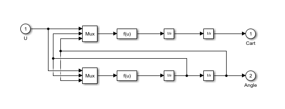
Here, the two Fcn blocks, with the mask label f(u), calculate the cart's linear acceleration and the pole's angular acceleration, respectively. The user-defined functions are derived from the mass-matrix equations previously discussed, where I, dF, and b are set to zero.

Derive the acceleration of the cart by using the mass-matrix representation.

D2x = diff(x(t),t,2) == simplify(subs(q_acc(1),[I dF b],[0 0 0]))

D2x = 
$$\frac{{\partial }^2}{\partial t^2}\mathrm{ }x\left(t\right)=\frac{-l\hspace{0.17em}m\hspace{0.17em}\sin \left(\theta \left(t\right)\right)\hspace{0.17em}{\left(\frac{\partial }{\partial t}\mathrm{ }\theta \left(t\right)\right)}^2+F+g\hspace{0.17em}m\hspace{0.17em}\cos \left(\theta \left(t\right)\right)\hspace{0.17em}\sin \left(\theta \left(t\right)\right)}{-m\hspace{0.17em}{\cos \left(\theta \left(t\right)\right)}^2+M+m}$$

Derive the angular acceleration of the pole by using the mass-matrix representation.

D2theta = diff(theta(t),t,2) == simplify(expand(subs(q_acc(2),[I dF b],[0 0 0])))

D2theta = 
$$\frac{{\partial }^2}{\partial t^2}\mathrm{ }\theta \left(t\right)=\frac{-l\hspace{0.17em}m\hspace{0.17em}\cos \left(\theta \left(t\right)\right)\hspace{0.17em}\sin \left(\theta \left(t\right)\right)\hspace{0.17em}{\left(\frac{\partial }{\partial t}\mathrm{ }\theta \left(t\right)\right)}^2+F\hspace{0.17em}\cos \left(\theta \left(t\right)\right)+M\hspace{0.17em}g\hspace{0.17em}\sin \left(\theta \left(t\right)\right)+g\hspace{0.17em}m\hspace{0.17em}\sin \left(\theta \left(t\right)\right)}{l\hspace{0.17em}\left(-m\hspace{0.17em}{\cos \left(\theta \left(t\right)\right)}^2+M+m\right)}$$

Examples of Cart-Pole System in Reinforcement Learning Toolbox

Reinforcement Learning Toolbox™ provides several cart-pole system environments, as described in Load Predefined Control System Environments (Reinforcement Learning Toolbox). The "CartPole-Discrete" and "CartPole-Continuous" environments are both available when you use the rlPredefinedEnv (Reinforcement Learning Toolbox) function. In these predefined environments, no force is applied to the pole ($$dF=0$$), the convention for $$\theta (t)$$ is reversed (the angle is positive for clockwise rotation instead of counterclockwise), and there is no friction ($$b=0$$). The pole is a uniform rod with a total length of $$2l$$, so the distance from the cart attachment to the pole's center of mass is $$l$$, and the pole's moment of inertia is $$\frac{1}{3}m{l}^2$$.

To derive the equations used in these environments, first use the first main equation in this example to obtain the acceleration of the cart by applying substitutions.

D2x = subs(isolate(mainEq1,diff(x(t),t,2)),[theta(t) dF b],[-theta(t) 0 0])

D2x = 
$$\frac{{\partial }^2}{\partial t^2}\mathrm{ }x\left(t\right)=\frac{F+l\hspace{0.17em}m\hspace{0.17em}\left(\sin \left(\theta \left(t\right)\right)\hspace{0.17em}{\left(\frac{\partial }{\partial t}\mathrm{ }\theta \left(t\right)\right)}^2-\cos \left(\theta \left(t\right)\right)\hspace{0.17em}\frac{{\partial }^2}{\partial t^2}\mathrm{ }\theta \left(t\right)\right)}{M+m}$$

Next, substitute the known parameter values into the second main equation.

mainEq2subs = subs(mainEq2,[theta(t) dF b I],[-theta(t) 0 0 1/3*m*l^2])

mainEq2subs(t) = 
$$\frac{4\hspace{0.17em}m\hspace{0.17em}{l}^2\hspace{0.17em}\frac{{\partial }^2}{\partial t^2}\mathrm{ }\theta \left(t\right)}{3}+m\hspace{0.17em}\cos \left(\theta \left(t\right)\right)\hspace{0.17em}l\hspace{0.17em}\frac{{\partial }^2}{\partial t^2}\mathrm{ }x\left(t\right)-g\hspace{0.17em}m\hspace{0.17em}\sin \left(\theta \left(t\right)\right)\hspace{0.17em}l=0$$

Substituting the expression of the cart acceleration results in this equation in terms of the angular acceleration of the pole.

thdd = collect(subs(mainEq2subs,lhs(D2x),rhs(D2x)),diff(theta(t),t,2))

thdd(t) = 
$$\left(\frac{4\hspace{0.17em}{l}^2\hspace{0.17em}m}{3}-\frac{l^2\hspace{0.17em}{m}^2\hspace{0.17em}{\cos \left(\theta \left(t\right)\right)}^2}{M+m}\right)\hspace{0.17em}\frac{{\partial }^2}{\partial t^2}\mathrm{ }\theta \left(t\right)-g\hspace{0.17em}l\hspace{0.17em}m\hspace{0.17em}\sin \left(\theta \left(t\right)\right)+\frac{l\hspace{0.17em}m\hspace{0.17em}\cos \left(\theta \left(t\right)\right)\hspace{0.17em}\left(l\hspace{0.17em}m\hspace{0.17em}\sin \left(\theta \left(t\right)\right)\hspace{0.17em}{\left(\frac{\partial }{\partial t}\mathrm{ }\theta \left(t\right)\right)}^2+F\right)}{M+m}=0$$

Dividing both terms of the previous equation by $$lm$$ yields the equation used in the code of the predefined environments. An alternative derivation of the system equations in this form is described in [2] and [3].

Examples of Cart-Pole System in Simscape Multibody

The Simulink-based reinforcement learning environments are implemented in Simscape Multibody within a Simulink model, using the architecture in the following diagram. This diagram differs from the block diagrams used in control systems, where the connecting lines represent physical connections instead of signals, and the blocks represent bodies, joints, sensors, and coordinate transformations instead of operations on the signals. Note that the force acting on the pole, dF, is positive in the x-direction, contrary to the convention that has been used throughout this example.

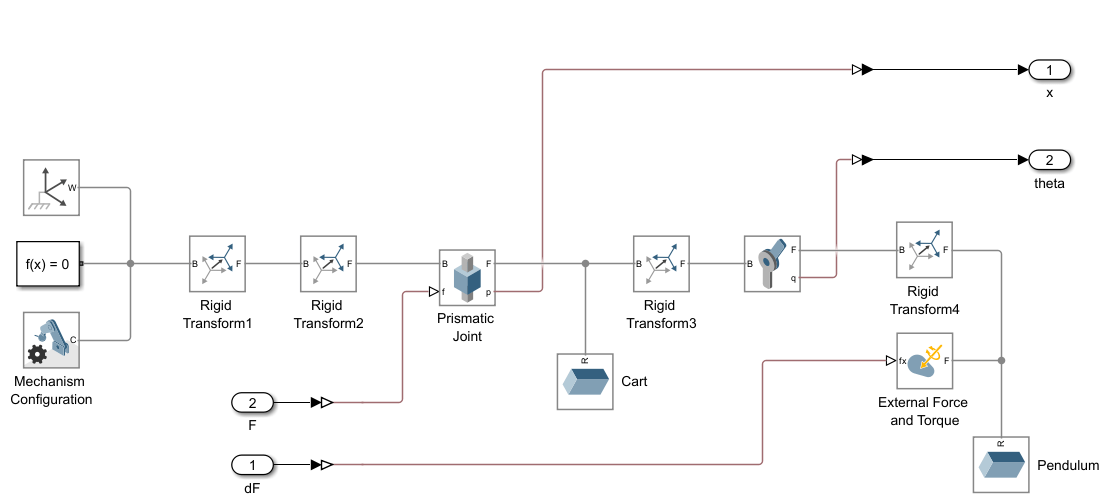
This Simscape Multibody model is used in the example Control of an Inverted Pendulum on a Cart (Simulink Control Design).

References

[1] Lunberg, Kent H., and Taylor W. Barton. "History of Inverted-Pendulum Systems". IFAC Proceedings Volumes, 8th IFAC Symposium on Advances in Control Education, 42, no. 24 (January 2010): 131–135. https://www.sciencedirect.com/science/article/pii/S1474667015316049.

[2] Florian, Răzvan V. "Correct equations for the dynamics of the cart-pole system". July 11, 2005; updated February 10, 2007. https://coneural.org/florian/papers/05_cart_pole.pdf.

[3] Green, Colin D. "Equations of Motion for the Cart and Pole Control Task". January 4, 2020. https://sharpneat.sourceforge.io/research/cart-pole/cart-pole-equations.html.

[4] "Inverted Pendulum". In Wikipedia, February 24, 2024. https://en.wikipedia.org/wiki/Inverted_pendulum.