FVTool

(제거될 예정임) 필터 시각화 툴

페이지 내 모두 확장

FVTool은 향후 릴리스에서 제거될 예정입니다. 필터 분석기를 대신 사용하십시오. 자세한 내용은 버전 내역 항목을 참조하십시오.

설명

필터 시각화 툴은 필터의 응답, 계수 및 기타 정보를 표시하고 분석할 수 있는 대화형 방식 앱입니다. FVTool과 필터 디자이너를 동기화하여 필터 설계에서 변경된 내용을 즉시 시각화할 수도 있습니다.

이 앱에서는 다음을 볼 수 있습니다.

크기 응답
위상 응답
군지연
위상 지연
임펄스 응답
계단 응답
극점-영점 플롯
필터 계수
필터 정보

자세한 내용은 분석 유형 항목을 참조하십시오.

자세히

DSP System Toolbox™가 설치되어 있는 경우 FVTool은 필터 System object™의 주파수 응답을 시각화할 수도 있습니다. 스트리밍 데이터를 실시간으로 필터링해야 하는 경우 System object를 사용하는 것이 좋습니다. 자세한 내용은 fvtool (DSP System Toolbox) 항목을 참조하십시오.

FVTool 열기

프로그래밍 방식 사용에 설명된 방법 중 하나를 사용하여 프로그래밍 방식으로 FVTool을 열 수 있습니다.

예제

모두 확장

타원 필터의 크기 응답

3dB의 통과대역 리플, 50dB의 저지대역 감쇠량, 1kHz의 샘플 레이트 및 300Hz의 정규화된 통과대역 경계를 갖는 6차 타원 필터가 있다고 가정하겠습니다. 필터의 크기 응답을 표시합니다.

[b,a] = ellip(6,3,50,300/500);
fvtool(b,a)

Magnitude response of an elliptic filter in FVTool.

프로그래밍 방식으로 사용

모두 확장

`fvtool(b,a)`

fvtool(b,a)는 FVTool을 열고 분자 b와 분모 a로 정의된 디지털 필터의 크기 응답을 표시합니다. b와 a 계수를 거듭제곱(z^-1)의 오름차순으로 지정합니다.

`fvtool(sos)`

fvtool(sos)는 FVTool을 열고 L×6 2차섹션형 행렬로 정의된 디지털 필터의 크기 응답을 표시합니다.

$sos = [\begin{matrix} b_{01} & b_{11} & b_{21} & 1 & a_{11} & a_{21} \\ b_{02} & b_{12} & b_{22} & 1 & a_{12} & a_{22} \\ ⋮ & ⋮ & ⋮ & ⋮ & ⋮ & ⋮ \\ b_{0 L} & b_{1 L} & b_{2 L} & 1 & a_{1 L} & a_{2 L} \end{matrix}]$

sos의 행에는 H(z)에 대한 2차섹션형 종속 연결의 분자 계수와 분모 계수인 b_ik와 a_ik가 포함되어 있습니다.

$H (z) = g \prod_{k = 1}^{L} H_{k} (z) = g \prod_{k = 1}^{L} \frac{b_{0 k} + b_{1 k} z^{- 1} + b_{2 k} z^{- 2}}{1 + a_{1 k} z^{- 1} + a_{2 k} z^{- 2}} .$

섹션 개수 L은 2보다 크거나 같아야 합니다. 섹션 개수가 2보다 작으면 fvtool이 입력값을 분자 벡터로 간주합니다.

`fvtool(d)`

fvtool(d)는 FVTool을 열고 디지털 필터 d의 크기 응답을 표시합니다. designfilt를 사용하여 주파수-응답 사양을 기반으로 d를 생성합니다.

`fvtool(b1,a1,b2,a2,...,bN,aN)`

fvtool(b1,a1,b2,a2,...,bN,aN)은 FVTool을 열고 분자 b1, …, bN과 분모 a1, ..., aN으로 정의된 여러 필터의 크기 응답을 표시합니다.

`fvtool(sos1,sos2,...,sosN)`

fvtool(sos1,sos2,...,sosN)은 FVTool을 열고 2차섹션형 행렬 sos1, sos2, ..., sosN으로 정의된 여러 필터의 크기 응답을 표시합니다.

`fvtool(Hd)`

fvtool(Hd)는 FVTool을 열고 dfilt 필터 객체 Hd 또는 dfilt 필터 객체의 배열에 대한 크기 응답을 표시합니다.

`fvtool(Hd1,Hd2,...,HdN)`

fvtool(Hd1,Hd2,...,HdN)은 FVTool을 열고 dfilt 객체 Hd1, Hd2, ...HdN에 포함된 필터의 크기 응답을 표시합니다.

`h = fvtool(___)`

h = fvtool(___)은 Figure 핸들 h를 반환합니다. 이 핸들을 사용하여 명령줄에서 FVTool과 상호 작용할 수 있습니다. 자세한 내용은 Controlling FVTool from the MATLAB Command Line 항목을 참조하십시오.

세부 정보

모두 확장

GUI에서 FVTool 제어

툴스트립에 있는 컨트롤을 사용하여 하나 또는 여러 개의 필터의 응답을 표시하고 분석합니다.

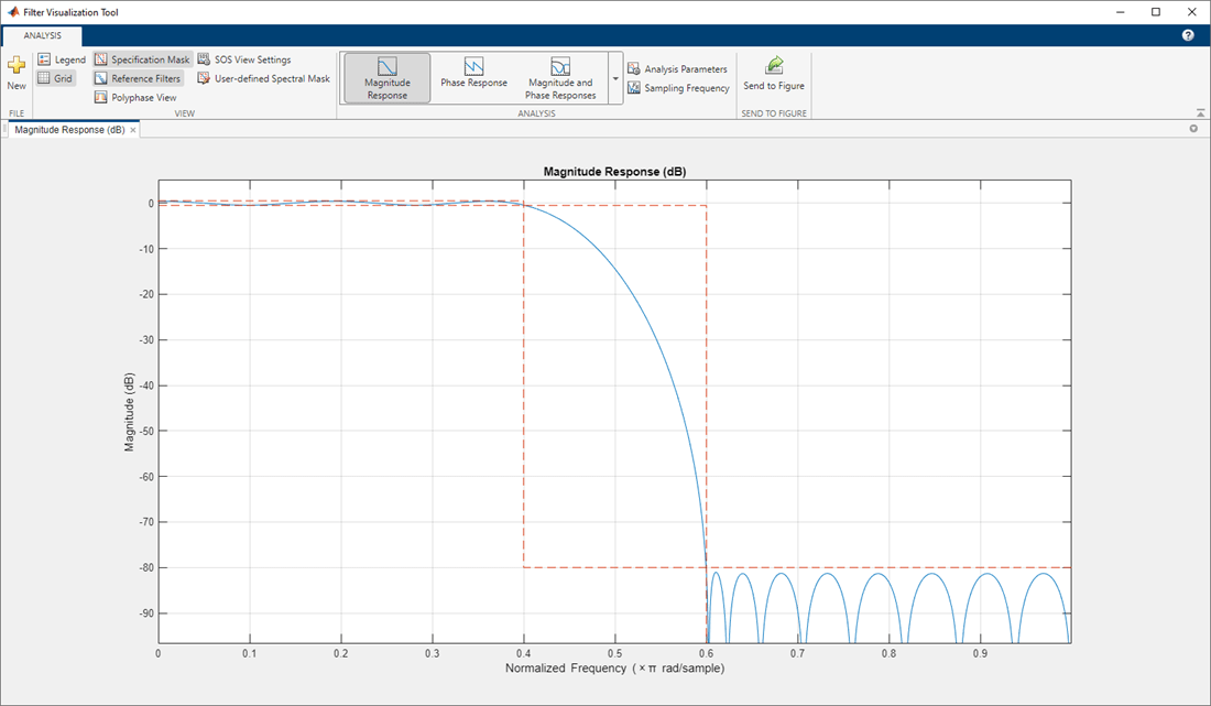
기본적으로 앱은 필터의 크기 응답을 표시합니다. 디스플레이를 변경하려면 툴스트립의 분석 섹션에 있는 분석 목록에서 옵션을 선택합니다.
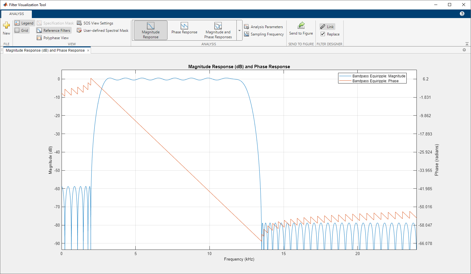
플롯에 두 번째 응답을 겹쳐 놓으려면 툴스트립의 분석 섹션에 있는 중첩 분석 목록에서 사용 가능한 응답을 선택합니다. 앱이 응답 플롯의 오른쪽에 두 번째 y축을 추가합니다. 분석 파라미터 대화 상자는 x축과 두 y축 모두에 대한 파라미터를 표시합니다.
보기 설정, 분석 파라미터를 조정하거나 샘플링 주파수를 지정하려면 툴스트립에서 해당하는 버튼을 사용합니다. 플롯 범례와 그리드를 켜거나 끌 수도 있습니다.
플롯을 편집하려면 먼저 Figure로 보내기를 클릭합니다. 새 Figure 창에서 플롯 편집 도구 모음을 사용하십시오.

Filter Visualization Tool

분석 유형

FVTool에는 다음과 같은 분석 유형이 있습니다.

분석	설명
크기 응답	영위상 응답을 보려면 플롯의 y축 레이블을 마우스 오른쪽 버튼으로 클릭하고 상황별 메뉴에서 영위상을 선택하십시오. 자세한 내용은 `freqz` 항목과 `zerophase` 항목을 참조하십시오.
위상 응답	자세한 내용은 `phasez` 항목을 참조하십시오.
크기 응답과 위상 응답	응답을 서로 겹쳐 놓습니다. 자세한 내용은 `freqz` 항목을 참조하십시오.
군지연	군지연은 주파수 함수 형태의, 필터에 대한 평균 지연입니다. 자세한 내용은 `grpdelay` 항목을 참조하십시오.
위상 지연	위상 지연은 필터가 입력 신호의 각 성분에 적용하는 시간 지연입니다. 자세한 내용은 `phasedelay` 항목을 참조하십시오.
임펄스 응답	임펄스 응답은 임펄스 입력값에 대한 필터의 응답입니다. 자세한 내용은 `impz` 항목을 참조하십시오.
계단 응답	계단 응답은 계단 입력값에 대한 필터의 응답입니다. 자세한 내용은 `stepz` 항목을 참조하십시오.
극점-영점 플롯	극점-영점 플롯은 z 평면에 필터의 극점 위치와 영점 위치를 표시합니다. 자세한 내용은 `zplane` 항목을 참조하십시오.
필터 계수	계수는 필터 구조(direct-form 또는 격자)에 따라 달라집니다. 텍스트 상자에 필터 계수가 표시됩니다. SOS 필터의 경우, 각 섹션이 별도의 필터로 표시됩니다.
필터 정보	필터 정보에는 필터의 구조, 위상, 안정성 및 구현 비용이 포함됩니다.

필터 디자이너에 연결하기

필터 디자이너 앱에 필터에 대한 분석이 표시될 때, 앱에서 보기 > 필터 시각화 툴 또는 전체 보기로 분석 도구 모음 버튼 을 선택하여 필터에 대한 FVTool을 엽니다. FVTool에서 연결 버튼을 사용하여 필터 디자이너에 연결합니다. FVTool은 필터 디자이너에서 필터에 대해 수행되는 모든 변경 사항으로 현재 디스플레이를 업데이트합니다. 기본적으로 앱은 현재 필터를 유지하고 새 필터를 디스플레이에 추가합니다. 현재 필터를 제거하고 새 필터를 삽입하려면 툴스트립의 필터 디자이너 섹션에서 바꾸기 체크박스를 선택하십시오.

버전 내역

R2006a 이전에 개발됨

모두 확장

R2024b: FVTool은 제거될 예정임

FVTool은 향후 릴리스에서 제거될 예정입니다. 필터 분석기를 대신 사용하십시오. 차이가 있어 코드를 업데이트해야 합니다.

다음과 같은 필터가 있다고 가정해 봅니다.

[b,a] = ellip(5,5,60,[0.2 0.45]);
dFd = designfilt("bandpassfir", ...
    SampleRate=2e3,PassbandRipple=5, ...
    StopbandFrequency1=500,PassbandFrequency1=600, ...
    StopbandAttenuation1=80, ...
    PassbandFrequency2=750,StopbandFrequency2=900, ...
    StopbandAttenuation2=40);

필터 분자 계수 b, 분모 계수 a, digitalFilter 객체 dFd가 주어진 경우 코드를 다음과 같이 업데이트해야 합니다.

R2024a 이하 버전의 원래 코드	R2024b에서 업데이트된 코드
fvtool(b,a,dFd)	filterAnalyzer(b,a,dFd)
fvtool(b,a,dFd,Analysis="freq")	filterAnalyzer(b,a,dFd, ... Analysis="magnitude",Overlay="phase")
fvtool(b,a,Fs=1000)	filterAnalyzer(b,a,SampleRates=1000)
fvtool(b,a,dFd,NumberofPoints=512, ... FrequencyRange="[0, 2pi)",FrequencyScale="Log")	filterAnalyzer(b,a,dFd,NFFT=512, ... FrequencyRange="twosided",FrequencyScale="log")
hfvt = fvtool(dFd); addfilter(hfvt,dfilt.df1(b,a))	fa = filterAnalyzer(dFd); addFilters(fa,b,a)
hfvt = fvtool(dFd); setfilter(hfvt,dfilt.df1(b,a))	fa = filterAnalyzer(dFd,FilterNames="df"); replaceFilters(fa,b,a,FilterNames="df")
hfvt = fvtool(b,a,dFd); deletefilter(hfvt,2)	fa = filterAnalyzer(b,a,dFd,FilterNames=["ba" "dFd"]); deleteFilters(fa,FilterNames="dFd")
hfvt = fvtool(b,a,dFd); legend(hfvt,"ba","dFd")	filterAnalyzer(b,a,dFd,FilterNames=["ba" "dFd"])
hfvt = fvtool(b,a,dFd); zoom(hfvt,[0.4 0.7 -30 0])	fa = filterAnalyzer(b,a,dFd); zoom(fa,"xy",[0.4 0.7 -30 0])
fvtool(b,a,dFd,Analysis="noisepower")	filterAnalyzer(b,a,dFd,Analysis="noisepsd")

필터 분석기에서는 2차섹션형(SOS) 형식이 지원되지 않습니다. 대신 종속 연결 전달 함수 형식을 사용하십시오. SOS 행렬 sos로 지정된 필터가 있는 경우, 코드를 다음과 같이 업데이트해야 합니다.

R2024a 이하 버전의 원래 코드	R2024b에서 업데이트된 코드
fvtool(sos)	filterAnalyzer(sos(:,1:3),sos(:,4:6)) 또는 [ctfNum,ctfDen] = sos2ctf(sos); filterAnalyzer(ctfNum,ctfDen)
hfvt = fvtool(sos); set(hfvt.SOSViewSettings,View="cumulative")	[ctfNum,ctfDen] = sos2ctf(sos); fa = filterAnalyzer(ctfNum,ctfDen,CTFAnalysisMode="cumulative");
hfvt = fvtool(sos); set(hfvt.SOSViewSettings,View="userdefined",UserDefined={3,1})	[ctfNum,ctfDen] = sos2ctf(sos); fa = filterAnalyzer(ctfNum,ctfDen, ... CTFAnalysisMode="specify",CTFAnalysisSections={3,1});

R2024a 이하 버전의 원래 코드

R2024b에서 업데이트된 코드

fvtool(sos)

filterAnalyzer(sos(:,1:3),sos(:,4:6))

또는

[ctfNum,ctfDen] = sos2ctf(sos);
filterAnalyzer(ctfNum,ctfDen)

hfvt = fvtool(sos);
set(hfvt.SOSViewSettings,View="cumulative")

[ctfNum,ctfDen] = sos2ctf(sos);
fa = filterAnalyzer(ctfNum,ctfDen,CTFAnalysisMode="cumulative");

hfvt = fvtool(sos);
set(hfvt.SOSViewSettings,View="userdefined",UserDefined={3,1})

[ctfNum,ctfDen] = sos2ctf(sos);
fa = filterAnalyzer(ctfNum,ctfDen, ...
    CTFAnalysisMode="specify",CTFAnalysisSections={3,1});

R2022a: 툴스트립에 컨트롤이 포함됨

FVTool의 동작이 변경되었습니다. 이전 릴리스에서는 앱에 플롯 편집 및 분석 도구 모음이 있었습니다. 이번 릴리스부터는 툴스트립에서 필터 시각화 컨트롤을 사용할 수 있습니다. 플롯을 편집하려면 먼저 플롯을 Figure로 내보낸 다음 Figure 컨트롤을 사용하십시오.

FVTool

설명

자세히

FVTool 열기

예제

타원 필터의 크기 응답

관련 예제

프로그래밍 방식으로 사용

`fvtool(b,a)`

`fvtool(sos)`

`fvtool(d)`

`fvtool(b1,a1,b2,a2,...,bN,aN)`

`fvtool(sos1,sos2,...,sosN)`

`fvtool(Hd)`

`fvtool(Hd1,Hd2,...,HdN)`

`h = fvtool(___)`

세부 정보

GUI에서 FVTool 제어

분석 유형

필터 디자이너에 연결하기

버전 내역

R2024b: FVTool은 제거될 예정임

R2022a: 툴스트립에 컨트롤이 포함됨

참고 항목

앱

함수

도움말 항목