주요 콘텐츠

phasedelay

R2026b

Phase delay of digital filter

Description

[phi,w] = phasedelay(b,a,n) returns the phase delay response of the specified digital filter. Specify a digital filter with numerator coefficients b and denominator coefficients a. The function returns the n-point phase delay response vector in phi and the corresponding angular frequency vector w.

[phi,w] = phasedelay(B,A,"ctf",n) returns the n-point phase delay response of the digital filter represented as Cascaded Transfer Functions (CTF) with numerator coefficients B and denominator coefficients A. (since R2024b)

example

[phi,w] = phasedelay({B,A,g},"ctf",n) returns the n-point phase delay response of the digital filter in CTF format. Specify the filter with numerator coefficients B, denominator coefficients A, and scaling values g across filter sections. (since R2024b)

example

[phi,w] = phasedelay(d,n) returns the n-point phase delay response of the digital filter d.

example

[phi,w] = phasedelay(sos,n) returns the n-point phase delay response corresponding to the second-order sections sos.

example

[phi,w] = phasedelay(___,n,"whole") returns the phase delay response at n equally spaced points around the whole unit circle.

example

[phi,f] = phasedelay(___,n,fs) returns the phase delay response and the corresponding n-point frequency vector f for a digital filter designed to filter signals sampled at a rate fs.

[phi,f] = phasedelay(___,n,"whole",fs) returns the frequency vector f at n points ranging between 0 and fs.

phi = phasedelay(___,w) returns the phase delay response evaluated at the angular frequencies specified in w.

example

phi = phasedelay(___,f,fs) returns the phase delay response evaluated at the frequencies specified in f.

[phi,w,s] = phasedelay(___) returns plotting information, where s is a structure with fields that you can change to display different frequency response plots.

[phi,f,s] = phasedelay(___) returns plotting information, where s is a structure with fields that you can change to display different frequency response plots.

phasedelay(___) plots the phase delay response versus frequency.

example

Examples

collapse all

Use constrained least squares to design a lowpass FIR filter of order 54 and normalized cutoff frequency 0.3. Specify the passband ripple and stopband attenuation as 0.02 and 0.08, respectively, expressed in linear units. Compute and plot the phase delay response of the filter.

Ap = 0.02;
As = 0.008;
b = fircls1(54,0.3,Ap,As);

phasedelay(b)
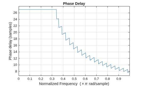
Figure contains an axes object. The axes object with title Phase Delay, xlabel Normalized Frequency ( times pi rad/sample), ylabel Phase delay (samples) contains an object of type line.

Repeat the example using designfilt. Express the passband ripple and stopband attenuation in decibels.

Apd = mag2db(((1+Ap)/(1-Ap))^2);
Asd = mag2db(1/As);
d = designfilt("lowpassfir",FilterOrder=54,CutoffFrequency=0.3, ...
    PassbandRipple=Apd,StopbandAttenuation=Asd);

phasedelay(d)
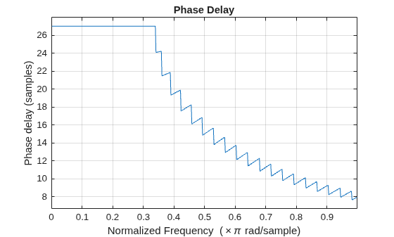
Figure contains an axes object. The axes object with title Phase Delay, xlabel Normalized Frequency ( times pi rad/sample), ylabel Phase delay (samples) contains an object of type line.

Since R2026b

The complex-valued frequency response of an order-Nlinear-phase FIR filter can be expressed as H(ejω)=A(ω)e-jωN/2, where A(ω) is a real-valued amplitude. The continuous (unwrapped) phase of H(ejω) is

H(ejω)={-ωN/2+2m/2π,A(ω)>0-ωN/2+(2m/2+1)π,A(ω)<0

where the winding number m is 0 at ω=0 and increases by 1 at each zero crossing of A(ω).

Then, the phase delay is

τp(ω)=-H(ejω)ω={N/2-2m/2π/ω,A(ω)>0N/2-(2m/2+1)π/ω,A(ω)<0

Design three lowpass FIR filters, each of them with a cutoff frequency ωn of 0.2π radians per sample. For each filter:

  • Plot the phase delay by using the phasedelay function.

  • Plot the phase by using the phasez function.

  • Plot the sign changes of A(ω) by using the zerophase and sign functions.

The filters show a constant phase delay within the passband region (ωωn).

Wn = 0.2;
N = [4 10 25];
tiledlayout("vertical")
for l = 1:numel(N)
    b = fir1(N(l),Wn);
    
    nexttile(1)
    phasedelay(b,1)
    ylabel("Samples")
    hold on
    
    nexttile(2)
    phasez(b,1)
    ylabel("Radians")
    hold on
    
    nexttile(3)
    [Hr,w] = zerophase(b,1);
    plot(w/pi,l+0.3*sign(Hr))
    grid on
    title("Change of +/– Sign of A(\omega)")
    xlabel("Normalized Frequency (\times\pi rad/sample)")
    set(gca,YTickLabel=[])
    y = find([0 diff(sign(Hr)')]~=0);
    text(-0.07,l,"m = ")
    text([0.01; w(y)/pi],l*ones(1+numel(y),1),string([0 cumsum(y.^0)]'))
    ylim([0 l+1])
    hold on
end
legend("N = " + N,Location="eastoutside")
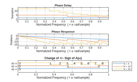
Figure contains 3 axes objects. Axes object 1 with title Phase Delay, xlabel Normalized Frequency (\times\pi rad/sample), ylabel Samples contains 3 objects of type line. Axes object 2 with title Phase Response, xlabel Normalized Frequency (\times\pi rad/sample), ylabel Radians contains 3 objects of type line. Axes object 3 with title Change of +/– Sign of A( omega ), xlabel Normalized Frequency (\times\pi rad/sample) contains 19 objects of type line, text. These objects represent N = 4, N = 10, N = 25.

Since R2024b

Design two digital IIR filters:

  • A 40th-order lowpass Chebyshev type II digital filter with a stopband edge frequency of 0.4 and stopband attenuation of 50 dB.

  • A 30th-order bandpass elliptic filter with passband edge frequencies of 0.3 and 0.7, passband ripple of 0.1 dB, and stopband attenuation of 50 dB.

Return the filter coefficients in the CTF format. For the elliptic filter, also return its gain.

[B1,A1] = cheby2(40,50,0.4,"ctf");
[B2,A2,g2] = ellip(30,0.1,50,[0.3 0.7],"ctf");

Plot the phase delay response of the filters using 1024 frequency points.

w = linspace(0,pi,512)';
phasedelay(B1,A1,"ctf",w)
hold on
phasedelay({B2,A2,g2},"ctf",w)
hold off
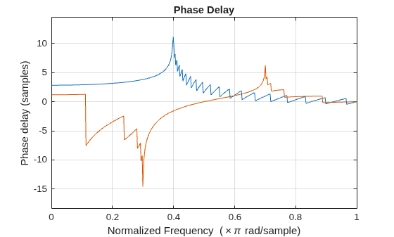
Figure contains an axes object. The axes object with title Phase Delay, xlabel Normalized Frequency ( times pi rad/sample), ylabel Phase delay (samples) contains 2 objects of type line.

Recalculate the phase delay of the filters using the definition.

τp(ω)=-H(ejω)ω

phi1 = phasez(B1,A1,"ctf",w);
phi2 = phasez({B2,A2,g2},"ctf",w);
pd = -[phi1 phi2]./w;
plot(w/pi,pd)
grid on
title("Phase Delay")
xlabel("Normalized Frequency (\times\pi rad/sample)")
ylabel("Phase delay (samples)")
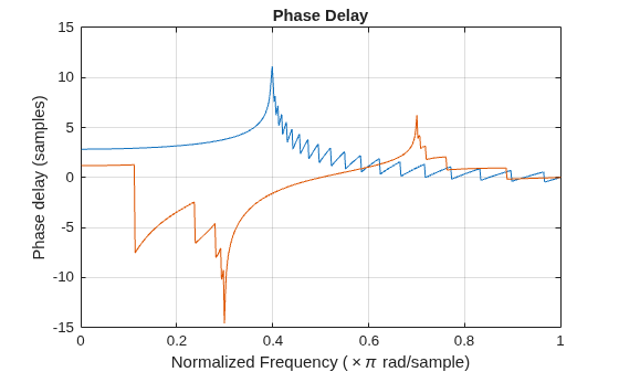
Figure contains an axes object. The axes object with title Phase Delay, xlabel Normalized Frequency ( times pi rad/sample), ylabel Phase delay (samples) contains 2 objects of type line.

Design a third-order lowpass Butterworth filter with a cutoff frequency of 200 Hz. The sample rate is 1000 Hz.

[B,A] = butter(3,200/(1000/2),"low","ctf");
sos = [B A];

Compute the phase delay response of the filter and set the number of evaluation points to 1024. Display the result.

phasedelay(sos,1024)
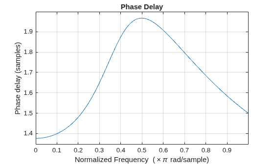
Figure contains an axes object. The axes object with title Phase Delay, xlabel Normalized Frequency ( times pi rad/sample), ylabel Phase delay (samples) contains an object of type line.

Design an elliptic filter of order 10 and normalized passband frequency 0.4. Specify a passband ripple of 0.5 dB and a stopband attenuation of 20 dB. Display the phase delay response of the filter over the complete unit circle.

[B,A] = ellip(10,0.5,20,0.4,"ctf");
phasedelay(B,A,512,"whole","ctf")
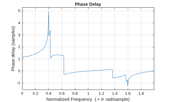
Figure contains an axes object. The axes object with title Phase Delay, xlabel Normalized Frequency ( times pi rad/sample), ylabel Phase delay (samples) contains an object of type line.

Repeat the example using designfilt.

d = designfilt("lowpassiir",DesignMethod="ellip", ...
               FilterOrder=10,PassbandFrequency=0.4, ...
               PassbandRipple=0.5,StopbandAttenuation=20);
phasedelay(d,512,"whole")
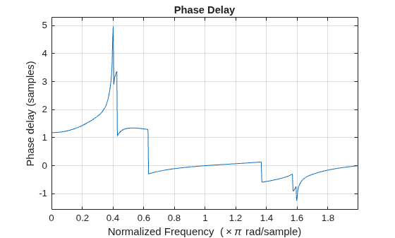
Figure contains an axes object. The axes object with title Phase Delay, xlabel Normalized Frequency ( times pi rad/sample), ylabel Phase delay (samples) contains an object of type line.

Since R2026b

Estimate and plot the phase delay of an IIR filter with numerator coefficients b and denominator coefficients a.

b = 0.05634*conv([1 1],[1 -1.0166 1]);
a = conv([1 -0.683],[1 -1.4461 +0.7959]);
phasedelay(b,a)
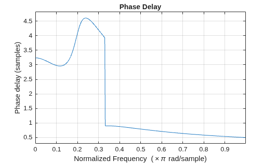
Figure contains an axes object. The axes object with title Phase Delay, xlabel Normalized Frequency ( times pi rad/sample), ylabel Phase delay (samples) contains an object of type line.

Extract the phase delay at the normalized frequencies of 0.1π, 0.2π, and 0.4π rad/sample.

wn = [0.1 0.2 0.4]';
pdFilter = phasedelay(b,a,wn*pi);

To compare the estimated phase delay of the IIR filter at these frequencies, filter a sinusoid with each of these normalized frequencies and estimate the delay (in samples) of the filtered signals.

n = (0:59);
x = sinpi(wn*n)';
y = filter(b,a,x);
pdFilteredSgn = finddelay(x,y);

Compare the filter phase delay and the signal delay in samples.

table(wn,pdFilteredSgn',round(pdFilter), ...
    VariableNames=["wn" "Filter Phase Delay" "Signal Delay"])
ans = 3×3 table
    wn     Filter Phase Delay    Signal Delay
    ___    __________________    ____________

    0.1            3                  3      
    0.2            4                  4      
    0.4            1                  1      

Input Arguments

collapse all

Transfer function coefficients, specified as vectors.

Data Types: single | double

Number of frequency points over which to evaluate response, specified as a positive integer. Set n to a value greater than the filter order.

Data Types: single | double

Cascaded transfer function (CTF) coefficients, specified as scalars, vectors, or matrices. B and A list the numerator and denominator coefficients of the cascaded transfer function, respectively.

B must be of size L-by-(m + 1) and A must be of size L-by-(n + 1), where:

  • L represents the number of filter sections.

  • m represents the order of the filter numerators.

  • n represents the order of the filter denominators.

For more information about the cascaded transfer function format and coefficient matrices, see Specify Digital Filters in CTF Format.

Note

If any element of A(:,1) is not equal to 1, then phasedelay normalizes the filter coefficients by A(:,1). In this case, A(:,1) must be nonzero.

Example: B = [2 4 2;3 3 0] and A = [6 0 2;6 0 0] specify a third-order Butterworth filter with normalized 3 dB frequency 0.5π rad/sample.

Data Types: double | single
Complex Number Support: Yes

Scale values, specified as a real-valued scalar or as a real-valued vector with L + 1 elements, where L is the number of CTF sections. The scale values represent the distribution of the filter gain across sections of the cascaded filter representation.

Depending on how you specify g, phasedelay applies a gain to the filter sections using the scaleFilterSections function:

  • Scalar — phasedelay distributes the gain uniformly across all filter sections.

  • Vector — phasedelay applies the first L gain values to the corresponding filter sections and distributes the last gain value uniformly across all filter sections.

Data Types: double | single

Digital filter, specified as a digitalFilter object. To generate d based on frequency-response specifications, use the designfilt function.

Second-order section coefficients, specified as a matrix. sos is a K-by-6 matrix, where K is the number of sections and must be greater than or equal to 2. If the number of sections is less than 2, the function considers the input to be a numerator vector, b. Each row of sos corresponds to the coefficients of a second-order (biquad) filter. The ith row of the sos matrix corresponds to [bi(1) bi(2) bi(3) ai(1) ai(2) ai(3)].

Data Types: single | double

Angular frequencies at which the function evaluates the phase delay response, specified as a vector and expressed in rad/sample. The frequencies are normally between 0 and π. w must contain at least two elements.

Sample rate, specified as a real-valued scalar and expressed in hertz.

Data Types: double

Frequencies at which the function evaluates the phase delay response, specified as a vector and expressed in hertz. f must contain at least two elements.

Output Arguments

collapse all

Phase delay response, returned as a vector of length n. The phase delay response is evaluated at n equally spaced points around the upper half of the unit circle.

Note

If the input to phasedelay is single precision, the function calculates the phase delay response using single-precision arithmetic. The output phi is single precision.

Angular frequencies in rad/sample, returned as a vector. If you specify n, w has length n. If you do not specify n or you specify n as an empty vector, then w has length 512.

Frequencies in hertz, returned as a vector. If you specify n, f has length n. If you do not specify n or you specify n as an empty vector, then f has length 512.

Plotting information, returned as a structure. You can modify the fields in s to display different frequency response plots.

More About

collapse all

Tips

You can obtain filters in CTF format, including the scaling gain. Use the outputs of digital IIR filter design functions, such as butter, cheby1, cheby2, and ellip. Specify the "ctf" filter-type argument in these functions and specify to return B, A, and g to get the scale values. (since R2024b)

Algorithms

The phase delay response of a filter corresponds to the time delay that each frequency component experiences as the input signal passes through the system. The phasedelay function returns the phase delay response and the frequency vector of the filter

H(ejω)=B(ejω)A(ejω)=b(1)+b(2)ejω++b(m+1)ejmωa(1)+a(2)ejω++a(n+1)ejnω

given numerator and denominator coefficients in inputs b and a.

Extended Capabilities

expand all

Version History

Introduced before R2006a

expand all