stftmag2sig
Signal reconstruction from STFT magnitude
Syntax
Description
x = stftmag2sig(s,nfft)x, estimated from
the Short-Time Fourier Transform (STFT) magnitude,
s, based on the Griffin-Lim algorithm. The function assumes
s was computed using discrete Fourier transform (DFT) length
nfft.
x = stftmag2sig(___,Name=Value)FrequencyRange="onesided",InitializePhaseMethod="random" specifies
that the signal is reconstructed from a one-sided STFT with random initial phases.
Examples
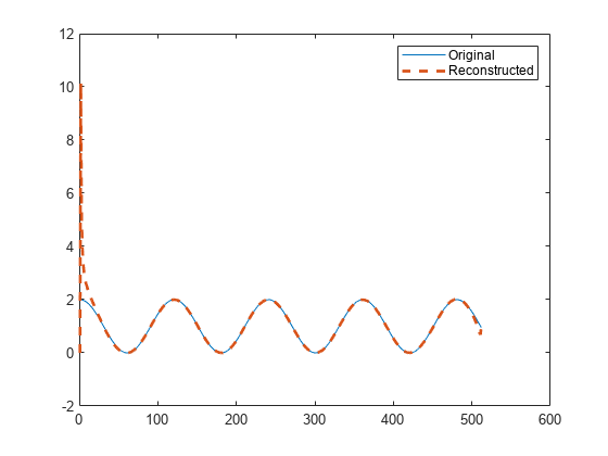
Consider 512 samples of a sinusoid with a normalized frequency of rad/sample and a DC value of 1. Compute the STFT of the signal.
n = 512;

x = cos(pi/60*(0:n-1)')+1;

S = stft(x);
Reconstruct the sinusoid from the magnitude of the STFT. Plot the original and reconstructed signals.
xr = stftmag2sig(abs(S),size(S,1));

plot(x)
hold on
plot(xr,"--",LineWidth=2)
hold off
legend("Original","Reconstructed")
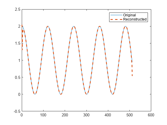
Repeat the computation, but now pad the signal with zeros to decrease edge effects.
xz = circshift([x; zeros(n,1)],n/2);

Sz = stft(xz);
xr = stftmag2sig(abs(Sz),size(Sz,1));

xz = xz(n/2+(1:n));
xr = xr(n/2+(1:n));

plot(xz)
hold on
plot(xr,"--",LineWidth=2)
hold off
legend("Original","Reconstructed")
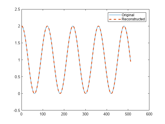
Repeat the computation, but now decrease edge effects by assuming that x is a segment of a signal twice as long.
xx = cos(pi/60*(-n/2:n/2+n-1)')+1;

Sx = stft(xx);
xr = stftmag2sig(abs(Sx),size(Sx,1));

xx = xx(n/2+(1:n));
xr = xr(n/2+(1:n));

plot(xx)
hold on
plot(xr,"--",LineWidth=2)
hold off
legend("Original","Reconstructed")
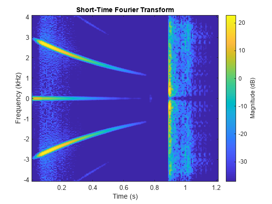
Load an audio signal that contains two decreasing chirps and a wideband splatter sound. The signal is sampled at 8192 Hz. Plot the STFT of the signal. Divide the waveform into 128-sample segments and window the segments using a Hamming window. Specify 64 samples of overlap between adjoining segments and 1024 DFT points.
load splat
ty = (0:length(y)-1)/Fs;

% To hear, type sound(y,Fs)

wind = hamming(128);
olen = 64;
nfft = 1024;

stft(y,Fs,Window=wind,OverlapLength=olen,FFTLength=nfft)
Compute the magnitude and phase of the STFT.
s = stft(y,Fs,Window=wind,OverlapLength=olen,FFTLength=nfft);

smag = abs(s);
sphs = angle(s);
Reconstruct the signal based on the magnitude of the STFT. Use the same parameters that you used to compute the STFT. By default, stftmag2sig initializes the phases to zero and uses 100 optimization iterations.
[x,tx,info] = stftmag2sig(smag,nfft,Fs, ...
    Window=wind,OverlapLength=olen);

% To hear the reconstruction, type sound(x,Fs)
Plot the original and reconstructed signals. For better comparison, shift the reconstructed signal vertically and to the right.
plot(ty,y,tx+500/Fs,x+1)
legend("Original","Reconstructed",Location="best")
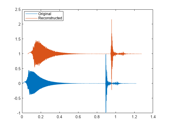
Output the relative improvement toward convergence between the last two iterations.
impr = info.Inconsistency
impr =
0.0579
Improve the reconstruction by doubling the number of optimization iterations and setting the initial phases to the actual phases from the STFT. Plot the original and reconstructed signals. For better comparison, plot the negative of the reconstructed signal and shift it vertically and to the right.
[x,tx,info] = stftmag2sig(smag,nfft,Fs, ...
    Window=wind,OverlapLength=olen, ...
    MaxIterations=200,InitialPhase=sphs);

% To hear the reconstruction, type sound(x,Fs)

plot(ty,y,tx+500/Fs,-x+1)
legend("Original","Reconstructed",Location="best")
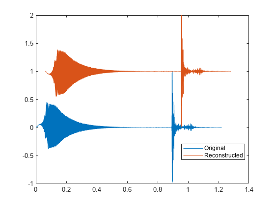
Output the relative improvement toward convergence between the last two iterations.
impr = info.Inconsistency
impr =
2.0299e-16
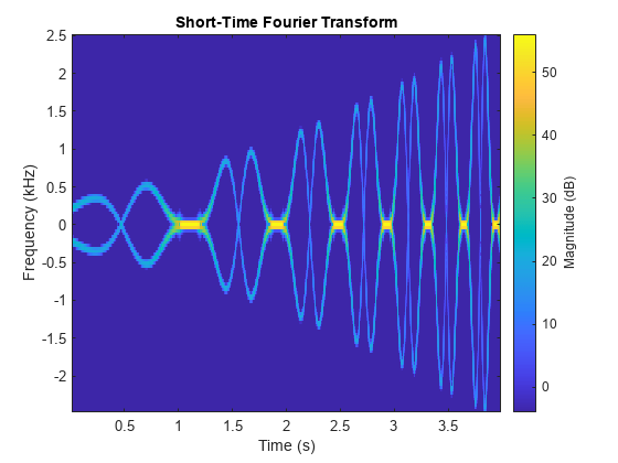
Generate a signal sampled at 5 kHz for 4 seconds. The signal consists of a set of pulses of decreasing duration separated by regions of oscillating amplitude and fluctuating frequency with an increasing trend.
fs = 5000;
t = 0:1/fs:4-1/fs;

x = 10*besselj(0,1000*(sin(2*pi*(t+2).^3/60).^5));
Compute and plot the short-time Fourier transform of the signal. Divide the signal into 128-sample segments and window the segments using a Hann window. Specify 96 samples of overlap between adjoining segments and 128 DFT points.
win = hann(128);
olen = 96;
nfft = 128;
stft(x,fs,Window=win,OverlapLength=olen,FFTLength=nfft)
Compute the magnitude and phase of the STFT.
s = stft(x,fs,Window=win,OverlapLength=olen,FFTLength=nfft);

smag = abs(s);
sphs = angle(s);
Reconstruct the signal based on the magnitude of the STFT. Use the same parameters that you used to compute the STFT. Instead of using the default Griffin-Lim algorithm, use the gradient descent method with the ADAM optimizer.
[xrec,trec,info] = stftmag2sig(smag,nfft,fs, ...
    Window=win,Method="gd",Optimizer="adam");
Plot the original and reconstructed signals. For better comparison, shift the reconstructed signal vertically so both are visible.
plot(t,x,trec,xrec+12)
legend("Original","Reconstructed",Location="northwest")
ylim([-5 27])

Compute the mean-squared error between the original signal and the reconstruction.
sum((x-xrec').^2)/length(x)
ans =
1.3620
For purposes of reproducibility, set the random seed to the default value. Generate 160 samples of a two-channel sinusoid. Add noise to each channel.
The first channel has unit amplitude and a normalized sinusoid frequency of rad/sample.
The second channel has unit amplitude and a normalized sinusoid frequency of rad/sample.
Compute the STFT of the signal. Divide the signal into 32-sample segments and window the segments using a Hann window.
rng default
N = 160;
t = 0:N-1;
win = hann(32);
signal = cos(pi./[4;2]*t)'+randn(N,2)/5;

s = stft(signal,Window=win);
Reconstruct the signal from the magnitude of the STFT. Use the gradient descent method with the L-BFGS optimizer. The L-BFGS optimizer automatically selects the step size for each iteration. Track the normalized inconsistency of each channel during the optimization process.
[x,tx,info] = stftmag2sig(abs(s), ...
    size(s,1),Window=win, ...
    Method="gd",Optimizer="lbfgs", ...
    Display=true);
#Iteration  |  Normalized Inconsistency
      1     |  1.2078e+00 1.2042e+00
     20     |  3.2348e-02 9.6221e-03
     40     |  1.9969e-02 6.8350e-03
     60     |  2.5463e-03 1.2099e-03
     80     |  2.4790e-03 8.4016e-04
    100     |  5.4774e-03 7.1804e-04

Decomposition process stopped.
The number of iterations reached the specified "MaxIterations" value of 100.
Plot the original and reconstructed signals.
tiledlayout(2,1)
nexttile
plot(t,signal(:,1))
hold on
plot(tx,x(:,1),"--",LineWidth=2)
hold off
title("First Channel")
legend("Original","Reconstructed", ...
    Location="northoutside")
nexttile
plot(t,signal(:,2))
hold on
plot(tx,x(:,2),"--",LineWidth=2)
hold off
title("Second Channel")
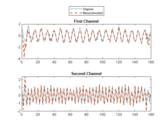
Output the relative improvement toward convergence between the last two iterations.
info.Inconsistency
ans = 1×2

    0.0055    0.0007
Input Arguments
Name-Value Arguments
Output Arguments
More About
Tips
If you are using the gradient descent method and the reconstruction is not satisfactory, set
Displaytotrue. Observe the inconsistency during iterations. If the inconsistency does not decrease, reduceStepSizefor better reconstruction.If you are using the gradient descent method, the L-BFGS optimizer usually provides the best results. This optimizer automatically selects the step size for each iteration. However, the L-BFGS optimizer may require more computation time than other optimizers to run the same number of iterations.
References
[1] Griffin, Daniel W., and Jae S. Lim. "Signal Estimation from Modified Short-Time Fourier Transform." IEEE Transactions on Acoustics, Speech, and Signal Processing. Vol. 32, Number 2, April 1984, pp. 236–243. https://doi.org/10.1109/TASSP.1984.1164317.
[2] Perraudin, Nathanaël, Peter Balazs, and Peter L. Søndergaard. "A Fast Griffin-Lim Algorithm." In 2013 IEEE Workshop on Applications of Signal Processing to Audio and Acoustics, New Paltz, NY, October 20–23, 2013. https://doi.org/10.1109/WASPAA.2013.6701851.
[3] Le Roux, Jonathan, Hirokazu Kameoka, Nobutaka Ono, and Shigeki Sagayama. "Fast Signal Reconstruction from Magnitude STFT Spectrogram Based on Spectrogram Consistency." In Proceedings of the 13th International Conference on Digital Audio Effects (DAFx-10), Graz, Austria, September 6–10, 2010.
[4] Ji, Li, and Zhou Tie. “On Gradient Descent Algorithm for Generalized Phase Retrieval Problem.” In 2016 IEEE 13th International Conference on Signal Processing (ICSP), 320–25. Chengdu, China: IEEE, 2016. https://doi.org/10.1109/ICSP.2016.7877848.