stftLayer
R2026bShort-time Fourier transform layer
Description
An STFT layer computes the short-time Fourier transform of the input. Use of this layer requires Deep Learning Toolbox™.
Creation
Description
layer = stftLayerstftLayer must be a real-valued dlarray (Deep Learning Toolbox) object in
"CBT" format with a size along the time dimension greater than the
length of Window. stftLayer formats the output as
"SCBT". For more information, see Layer Output Format.
Note
When you initialize the learnable parameters of stftLayer, the
layer weights are set to the analysis window used to compute the transform. It is not
recommended to initialize the weights directly.
layer = stftLayer(PropertyName=Value)
Note
You cannot use this syntax to set the Weights
property.
Example: stfl =
stftLayer(Window=triang(64),OverlapLength=48,FFTLength=512) creates an STFT
layer with a 64-sample triangular window, 48 samples of overlap between adjoining windows,
and 512 DFT points.
Properties
Examples
Generate a signal sampled at 600 Hz for 2 seconds. The signal consists of a chirp with sinusoidally varying frequency content. Store the signal in a deep learning array with "CTB" format.
fs = 6e2;
x = vco(sin(2*pi*(0:1/fs:2)),[0.1 0.4]*fs,fs);

dlx = dlarray(x,"CTB");
Create a short-time Fourier transform layer with default properties. Create a dlnetwork object consisting of a sequence input layer and the short-time Fourier transform layer. Specify a minimum sequence length of 128 samples. Run the signal through the predict method of the network.
ftl = stftLayer;

dlnet = dlnetwork([sequenceInputLayer(1,MinLength=128) ftl]);
netout = predict(dlnet,dlx);
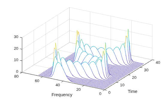
Convert the network output to a numeric array. Use the squeeze function to remove the length-1 channel and batch dimensions. Plot the magnitude of the STFT. The first dimension of the array corresponds to frequency and the second to time.
q = extractdata(netout);

waterfall(squeeze(q)')
set(gca,XDir="reverse",View=[30 45])
xlabel("Frequency")
ylabel("Time")
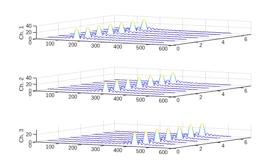
Generate a 3 × 160 (× 1) array containing one batch of a three-channel, 160-sample sinusoidal signal. The normalized sinusoid frequencies are π/4 rad/sample, π/2 rad/sample, and 3π/4 rad/sample. Save the signal as a dlarray, specifying the dimensions in order. dlarray permutes the array dimensions to the "CBT" shape expected by a deep learning network.
nch = 3;
N = 160;
x = dlarray(cos(pi.*(1:nch)'/4*(0:N-1)),"CTB");
Create a short-time Fourier transform layer that can be used with the sinusoid. Specify a 64-sample rectangular window, 48 samples of overlap between adjoining windows, and 1024 DFT points. By default, the layer outputs the magnitude of the STFT.
stfl = stftLayer(Window=rectwin(64),OverlapLength=48,FFTLength=1024);
Create a two-layer dlnetwork object containing a sequence input layer and the STFT layer you just created. Treat each channel of the sinusoid as a feature. Specify the signal length as the minimum sequence length for the input layer.
layers = [sequenceInputLayer(nch,MinLength=N) stfl];
dlnet = dlnetwork(layers);
Run the sinusoid through the forward method of the network.
dataout = forward(dlnet,x);
Convert the network output to a numeric array. Use the squeeze function to collapse the size-1 batch dimension. Permute the channel and time dimensions so that each array page contains a two-dimensional spectrogram. Plot the STFT magnitude separately for each channel in a waterfall plot.
q = squeeze(extractdata(dataout));
q = permute(q,[1 3 2]);

tiledlayout("vertical")
for kj = 1:nch
    nexttile
    waterfall(q(:,:,kj)')
    view(30,45)
    zlabel("Ch. " + kj)
end
Create a deep learning network that demonstrates perfect reconstruction of the short-time Fourier transform (STFT) of a deep learning array. To minimize edge effects, the network zero-pads the data before computing the STFT.
Generate a 3-by-2000-by-5 array containing five batches of a three-channel sinusoidal signal sampled at 1 kHz for two seconds. Save the array as a dlarray, specifying the dimensions in order. dlarray permutes the array dimensions to the "CBT" shape expected by a deep learning network. Display the array dimension sizes.
Fs = 1e3;
nchan = 3;
nbtch = 5;
nsamp = 2000;
t = (0:nsamp-1)/Fs;

x = zeros(nchan,nsamp,nbtch);
for k=1:nbtch
    x(:,:,k) = sin(k*pi.*(1:nchan)'*t)+cos(k*pi.*(1:nchan)'*t);
end

xd = dlarray(x,"CTB");
Design a periodic Hann window of length 100 and set the number of overlap samples to 75. Check the window and overlap length for COLA compliance.
nwin = 100;
win = hann(nwin,"periodic");
noverlap = 75;

tf = iscola(win,noverlap)
tf = logical
1
Create a STFT layer and an ISTFT layer using the stftLayer and istftLayer objects, respectively.
For both layers, use the Hann window and number of overlap samples. Set the FFT length to 128.
To concatenate the real and imaginary parts of the STFT layer output along the channel dimension, set the layer transform mode to
"realimag"in thestftLayerobject.To apply weight tying, set the
OutputLearnablesandInputLearnablesproperties to"Weights"in thestftLayerandistftLayerobject, respectively.
fftlen = 128;

ftl = stftLayer(Window=win,FFTLength=fftlen, ...
    OverlapLength=noverlap,TransformMode="realimag", ...
    Name="stft",OutputLearnables="Weights");

iftl = istftLayer(Window=win,FFTLength=fftlen, ...
    OverlapLength=noverlap, ...
    Name="istft",InputLearnables="Weights");
Create a deep learning network appropriate for the data that demonstrates perfect reconstruction of the STFT. Use a function layer to zero-pad the data on both sides along the time dimension before computing the STFT. The length of the zero padding is the window length. Use a function layer after the ISTFT layer to trim both sides of the ISTFT layer output by the same amount. To complete the weight tying, connect the STFT and ISTFT layers.
layers = [
    sequenceInputLayer(nchan,MinLength=nsamp)
    functionLayer(@(X) paddata(X,nsamp+2*nwin,dimension=3,side="both"))
    ftl
    iftl
    functionLayer(@(X) trimdata(X,nsamp,dimension=3,side="both"))];
dlnet = dlnetwork(layers,Initialize=false);
dlnet = connectLayers(dlnet,"stft/Weights","istft/Weights");
dlnet = initialize(dlnet);
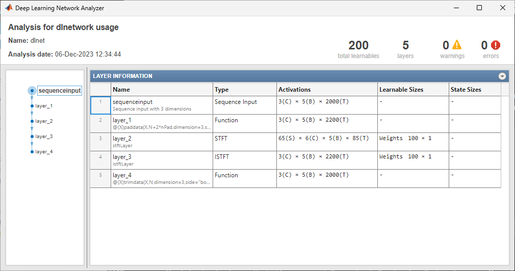
Analyze the network using the data. The number of channels of the STFT layer output is twice the layer input.
analyzeNetwork(dlnet,xd)
Run the data through the forward method of the network.
dataout = forward(dlnet,xd);
The output is a dlarray object in "CBT" format. Convert the network output to a numeric array. Permute the dimensions so that each page is a batch.
xrec = extractdata(dataout);
xrec = permute(xrec,[1 3 2]);
Choose a batch. Plot the original and reconstructed multichannel signal of that batch as a stacked plot.
wb = 4;
tiledlayout(2,1)
nexttile
stackedplot(x(:,:,wb)',DisplayLabels="Channel "+string(1:nchan))
title("Batch "+num2str(wb)+": Original")
nexttile
stackedplot(xrec(:,:,wb)',DisplayLabels="Channel "+string(1:nchan))
title("Batch "+num2str(wb)+": Reconstruction")
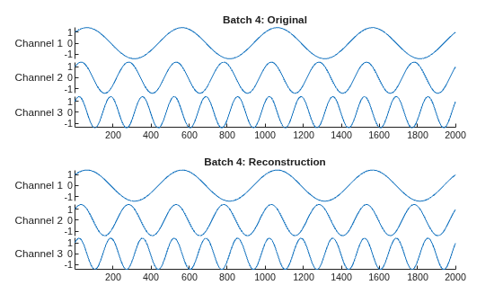
Confirm perfect reconstruction of the data.
max(abs(x(:)-xrec(:)))
ans = single

5.6394e-07
Since R2025a
Verify that the weights of a short-time Fourier transform (STFT) layer are reset to the specified window when you reinitialize the containing network.
Define an array of seven layers: a sequence input layer, an STFT layer, a 2-D convolutional layer, a batch normalization layer, a rectified linear unit (ReLU) layer, a fully connected layer, and a softmax layer. There is one feature in the sequence input. Set the minimum signal length in the sequence input layer to 512 samples. For the STFT layer, use a 256-sample Hamming window and an overlap length of 128 samples.
win = hamming(256);
layers = [
   sequenceInputLayer(1,MinLength=512)
   stftLayer(Window=win,OverlapLength=128,Name="stft")
   convolution2dLayer(4,16,Padding="same")
   batchNormalizationLayer
   reluLayer
   fullyConnectedLayer(3)
   softmaxLayer];
Create a deep learning neural network from the layer array. By default, the dlnetwork function initializes the network at creation. For reproducibility, use the default random number generator.
rng("default")
net = dlnetwork(layers);
Display the table of learnable parameters. The network weights and bias are nonempty dlarray objects.
tInit1 = net.Learnables
tInit1 = 7×3 table
       Layer       Parameter           Value
    ___________    _________    ____________________

    "stft"         "Weights"    {256×1      dlarray}
    "conv"         "Weights"    {  4×4×1×16 dlarray}
    "conv"         "Bias"       {  1×1×16   dlarray}
    "batchnorm"    "Offset"     {  1×16     dlarray}
    "batchnorm"    "Scale"      {  1×16     dlarray}
    "fc"           "Weights"    {  3×2064   dlarray}
    "fc"           "Bias"       {  3×1      dlarray}
Compare the initialized weights of the STFT layer from the list of learnable parameters with the Window property of the STFT layer. The stftLayer weights are single precision and initialized to the specified window.
isequal(tInit1.Value{1},single(net.Layers(2).Window))ans = logical
1
Set the learnable parameters to empty arrays. Reinitialize the network. Display the network and the learnable parameters. The network weights and bias are nonempty dlarray objects.
net = dlupdate(@(x)[],net);
net = initialize(net);
tInit2 = net.Learnables
tInit2 = 7×3 table
       Layer       Parameter           Value
    ___________    _________    ____________________

    "stft"         "Weights"    {256×1      dlarray}
    "conv"         "Weights"    {  4×4×1×16 dlarray}
    "conv"         "Bias"       {  1×1×16   dlarray}
    "batchnorm"    "Offset"     {  1×16     dlarray}
    "batchnorm"    "Scale"      {  1×16     dlarray}
    "fc"           "Weights"    {  3×2064   dlarray}
    "fc"           "Bias"       {  3×1      dlarray}
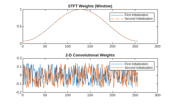
Compare the weights from the STFT and 2-D convolutional layers along the two initialization calls. The STFT layer sets the weights using the specified window, while the convolutional layer weights consists of a new set of random values.
tiledlayout flow
nexttile
plot(tInit1.Value{1})
hold on
plot(tInit2.Value{1},"--")
hold off
title("STFT Weights (Window)")
legend(["First" "Second"] + " Initialization")
nexttile
plot([tInit1.Value{2}(:) tInit2.Value{2}(:)])
title("2-D Convolutional Weights")
legend(["First" "Second"] + " Initialization")
More About
Extended Capabilities
Version History
Introduced in R2021bSee Also
Apps
- Deep Network Designer (Deep Learning Toolbox)
Objects
istftLayer|dlarray(Deep Learning Toolbox) |dlnetwork(Deep Learning Toolbox)
Functions
dlstft|stft|dlistft|istft|stftmag2sig

