Learn Pre-Emphasis Filter Using Deep Learning

Since R2021b

This example shows how to use a convolutional deep network to learn a pre-emphasis filter for speech recognition. The example uses a learnable short-time Fourier transform (STFT) layer to obtain a time-frequency representation suitable for use with 2-D convolutional layers. The use of a learnable STFT enables a gradient-based optimization of the pre-emphasis filter weights.

Data

Download the Free Spoken Digit Data Set (FSDD)[1]. FSDD is an open data set, which means that it can grow over time. This example uses the version committed on November 13, 2019, which consists of 2000 recordings in English of the digits 0 through 9 obtained from six speakers. Each digit is spoken 50 times by each speaker. The data is sampled at 8000 Hz.

downloadFolder = matlab.internal.examples.downloadSupportFile("audio","FSDD.zip");
dataFolder = tempdir;
unzip(downloadFolder,dataFolder)
dataset = fullfile(dataFolder,"FSDD");

Create an audioDatastore that points to the dataset.

ads = audioDatastore(dataset,IncludeSubfolders=true);

Use the filenames2labels function to obtain a categorical vector of labels from the FSDD files. Display the count of each label in the data set.

lbls = filenames2labels(ads,ExtractBefore="_");
ads.Labels = lbls;
countlabels(lbls)

ans=10×3 table
    0    200    10
    1    200    10
    2    200    10
    3    200    10
    4    200    10
    5    200    10
    6    200    10
    7    200    10
    8    200    10
    9    200    10

Split the FSDD into training and test sets maintaining equal class proportions in each subset. For reproducible results, set the random number generator to its default value. Use 80%, or 1600 recordings, for training. The remaining 400 recordings, 20% of the total, are held out for testing. Shuffle the files in the datastore once before creating the training and test sets.

rng default;
ads = shuffle(ads);
[adsTrain,adsTest] = splitEachLabel(ads,0.8,0.2);

The recordings in FSDD are not equal in length. Use a transform so that each read from the datastore is padded or truncated to 8192 samples. The data are additionally cast to single-precision and a z-score normalization is applied.

transTrain = transform(adsTrain,@(x,info)helperReadData(x,info),'IncludeInfo',true);
transTest = transform(adsTest,@(x,info)helperReadData(x,info),'IncludeInfo',true);

Deep Convolutional Neural Network (DCNN) Architecture

This example uses a custom training loop with the following deep convolutional network.

numF = 12;
dropoutProb = 0.2;
layers = [
    sequenceInputLayer(1,'Name','input','MinLength',8192,...
         'Normalization',"none")

    convolution1dLayer(5,1,"name","pre-emphasis-filter",...
    "WeightsInitializer",@(sz)kronDelta(sz),"BiasLearnRateFactor",0)  

    stftLayer('Window',hamming(1280),'OverlapLength',900,...
    'Name','STFT') 
    
    convolution2dLayer(5,numF,'Padding','same')
    batchNormalizationLayer
    reluLayer

    maxPooling2dLayer(3,'Stride',2,'Padding','same')

    convolution2dLayer(3,2*numF,'Padding','same')
    batchNormalizationLayer
    reluLayer

    maxPooling2dLayer(3,'Stride',2,'Padding','same')

    convolution2dLayer(3,2*numF,'Padding','same')
    batchNormalizationLayer
    reluLayer

    maxPooling2dLayer(3,'Stride',2,'Padding','same')

    convolution2dLayer(3,4*numF,'Padding','same')
    batchNormalizationLayer
    reluLayer

    maxPooling2dLayer(3,'Stride',2,'Padding','same')

    convolution2dLayer(3,4*numF,'Padding','same')
    batchNormalizationLayer
    reluLayer

    maxPooling2dLayer(3,'Stride',2,'Padding','same')

    convolution2dLayer(3,4*numF,'Padding','same')
    batchNormalizationLayer
    reluLayer

    maxPooling2dLayer(3,'Stride',2,'Padding','same')

    convolution2dLayer(3,4*numF,'Padding','same')
    batchNormalizationLayer
    reluLayer

    maxPooling2dLayer(3,'Stride',2,'Padding','same')

    convolution2dLayer(3,4*numF,'Padding','same')
    batchNormalizationLayer
    reluLayer

    maxPooling2dLayer(3,'Stride',2,'Padding','same')
    
    convolution2dLayer(3,4*numF,'Padding','same')
    batchNormalizationLayer
    reluLayer

    maxPooling2dLayer(3,'Stride',2,'Padding','same')
   
    convolution2dLayer(3,4*numF,'Padding','same')
    batchNormalizationLayer
    reluLayer

    maxPooling2dLayer(3,'Stride',2,'Padding','same')

    convolution2dLayer(3,4*numF,'Padding','same')
    batchNormalizationLayer
    reluLayer

    maxPooling2dLayer(3,'Stride',2,'Padding','same')

    convolution2dLayer(3,4*numF,'Padding','same')
    batchNormalizationLayer
    reluLayer

    dropoutLayer(dropoutProb)
    globalAveragePooling2dLayer
    fullyConnectedLayer(numel(categories(ads.Labels)))
    softmaxLayer    
    ];
dlnet = dlnetwork(layers);

The sequence input layer is followed by a 1-D convolution layer consisting of a single filter with 5 coefficients. This is a finite impulse response filter. Convolutional layers in deep learning networks by default implement an affine operation on the input features. To obtain a strictly linear (filtering) operation, use the default 'BiasInitializer' which is 'zeros' and set the bias learn rate factor of the layer to 0. This means that the bias is initialized to 0 and never changes during training. The network uses a custom initialization of the filter weights to be a scaled Kronecker delta sequence. This is an allpass filter, which performs no filtering of the input. The code for the allpass filter weight initializer is shown here.

function delta = kronDelta(sz)
% This function is only for use in the "Learn Pre-Emphasis Filter using
% Deep Learning" example. It may change or be removed in a
% future release.

L = sz(1);
delta = zeros(L,sz(2),sz(3),'single');
delta(1) = 1/sqrt(L);

end

stftLayer takes the filtered batch of input signals and obtains their magnitude STFTs. The magnitude STFT is a 2-D representation of the signal, which is amenable to use in 2-D convolutional networks.

While the weights of the STFT are not changed here during training, the layer supports backpropagation, which enables the filter coefficients in the "pre-emphasis-filter" layer to be learned.

Network Training

Set the training options for the custom training loop. Use 70 epochs with a minibatch size of 128. Set the initial learn rate to 0.001.

NumEpochs = 70;
miniBatchSize = 128;
learnRate = 0.001;

In the custom training loop, use a minibatchqueue object. The processSpeechMB function reads in a minibatch and applies a one-hot encoding scheme to the labels.

mbqTrain = minibatchqueue(transTrain,2,...
    'MiniBatchSize',miniBatchSize,...
    'MiniBatchFormat', {'CBT','CB'}, ... 
    'MiniBatchFcn', @processSpeechMB);

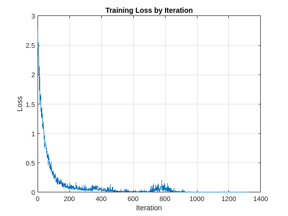
Train the network and plot the loss for each iteration. Use an Adam optimizer to update the network learnable parameters. To plot the loss as training progress, set the value of progress in the following code to "training-progress".

progress = "final-loss";
if progress == "training-progress"
    figure
    lineLossTrain = animatedline;
    ylim([0 inf])
    xlabel("Iteration")
    ylabel("Loss")
    grid on
end

% Initialize some training loop variables
trailingAvg = [];
trailingAvgSq = [];
iteration = 0;
lossByIteration = 0;

% Loop over epochs and time the epochs
start = tic;

for epoch = 1:NumEpochs
    reset(mbqTrain)
    shuffle(mbqTrain)

    % Loop over mini-batches
    while hasdata(mbqTrain)
        iteration = iteration + 1;
        
        % Get the next minibatch and one-hot coded targets
        [dlX,Y] = next(mbqTrain);
        
        % Evaluate the model gradients and loss 
        [gradients, loss, state] = dlfeval(@modelGradSTFT,dlnet,dlX,Y);
        if progress == "final-loss"
            lossByIteration(iteration) = loss;
        end

        % Update the network state
        dlnet.State = state;
        
        % Update the network parameters using an Adam optimizer
        [dlnet,trailingAvg,trailingAvgSq] = adamupdate(...
            dlnet,gradients,trailingAvg,trailingAvgSq,iteration,learnRate);        
        
        % Display the training progress
        D = duration(0,0,toc(start),'Format','hh:mm:ss');
        if progress == "training-progress"
            addpoints(lineLossTrain,iteration,loss)
            title("Epoch: " + epoch + ", Elapsed: " + string(D))
        end
        
    end
    disp("Training loss after epoch " + epoch + ": " + loss); 

end

Training loss after epoch 1: 1.6652
Training loss after epoch 2: 1.1411
Training loss after epoch 3: 0.78417
Training loss after epoch 4: 0.63184
Training loss after epoch 5: 0.48744
Training loss after epoch 6: 0.39178
Training loss after epoch 7: 0.26968
Training loss after epoch 8: 0.28975
Training loss after epoch 9: 0.15348
Training loss after epoch 10: 0.22781
Training loss after epoch 11: 0.2057
Training loss after epoch 12: 0.17013
Training loss after epoch 13: 0.10964
Training loss after epoch 14: 0.10967
Training loss after epoch 15: 0.091592
Training loss after epoch 16: 0.094693
Training loss after epoch 17: 0.044116
Training loss after epoch 18: 0.1126
Training loss after epoch 19: 0.069462
Training loss after epoch 20: 0.11456
Training loss after epoch 21: 0.11415
Training loss after epoch 22: 0.06416
Training loss after epoch 23: 0.11352
Training loss after epoch 24: 0.038266
Training loss after epoch 25: 0.076066
Training loss after epoch 26: 0.050454
Training loss after epoch 27: 0.019133
Training loss after epoch 28: 0.028106
Training loss after epoch 29: 0.012322
Training loss after epoch 30: 0.021237
Training loss after epoch 31: 0.016239
Training loss after epoch 32: 0.012996
Training loss after epoch 33: 0.01065
Training loss after epoch 34: 0.0079017
Training loss after epoch 35: 0.012452
Training loss after epoch 36: 0.010239
Training loss after epoch 37: 0.014491
Training loss after epoch 38: 0.012002
Training loss after epoch 39: 0.015212
Training loss after epoch 40: 0.010369
Training loss after epoch 41: 0.017623
Training loss after epoch 42: 0.0040403
Training loss after epoch 43: 0.010414
Training loss after epoch 44: 0.007087
Training loss after epoch 45: 0.0089144
Training loss after epoch 46: 0.0080485
Training loss after epoch 47: 0.0049819
Training loss after epoch 48: 0.0068432
Training loss after epoch 49: 0.0043644
Training loss after epoch 50: 0.0033179
Training loss after epoch 51: 0.0049078
Training loss after epoch 52: 0.0031546
Training loss after epoch 53: 0.0046745
Training loss after epoch 54: 0.0057065
Training loss after epoch 55: 0.0062487
Training loss after epoch 56: 0.0069303
Training loss after epoch 57: 0.0027477
Training loss after epoch 58: 0.0031618
Training loss after epoch 59: 0.0040211
Training loss after epoch 60: 0.0067042
Training loss after epoch 61: 0.0058158
Training loss after epoch 62: 0.0037038
Training loss after epoch 63: 0.0064653
Training loss after epoch 64: 0.0058798
Training loss after epoch 65: 0.0043404
Training loss after epoch 66: 0.003792
Training loss after epoch 67: 0.0026022
Training loss after epoch 68: 0.005193
Training loss after epoch 69: 0.0032368
Training loss after epoch 70: 0.0038476

if progress == "final-loss"
        plot(1:iteration,lossByIteration)
        grid on 
        title('Training Loss by Iteration')
        xlabel("Iteration")
        ylabel("Loss")
end

Test the trained network on the held-out test set. Use a minibatchqueue object with a minibatch size of 32.

miniBatchSize = 32;
mbqTest = minibatchqueue(transTest,2,...
    'MiniBatchSize',miniBatchSize,...
    'MiniBatchFormat', {'CBT','CB'}, ... 
    'MiniBatchFcn', @processSpeechMB);

Loop over the test set and predict the class labels for each minibatch.

numObservations = numel(adsTest.Files);
classes = string(unique(adsTest.Labels));

predictions = [];

% Loop over mini-batches
while hasdata(mbqTest)    
    % Read mini-batch of data
    dlX = next(mbqTest);

    % Make predictions on the minibatch
    dlYPred = predict(dlnet,dlX);

    % Determine corresponding classes
    predBatch = onehotdecode(dlYPred,classes,1);
    predictions = [predictions predBatch];  
end

Evaluate the classification accuracy on the 400 examples in the held-out test set.

accuracy = mean(predictions' == categorical(adsTest.Labels))

accuracy = 
0.9650

Test performance is approximately 99%. You can comment out the 1-D convolution layer and retrain the network without the pre-emphasis filter. The test performance without the pre-emphasis filter is also excellent at approximately 96%, but the use of the pre-emphasis filter makes a small improvement. It is noteworthy, that while the use of the learned pre-emphasis filter has only improved the test accuracy slightly, this was achieved by adding only 5 learnable parameters to the network.

To examine the learned pre-emphasis filter, extract the weights of the 1-D convolutional layer. Plot the frequency response. Recall that the sampling frequency of the data is 8 kHz. Because we initialized the filter to a scaled Kronecker delta sequence (allpass filter), we can easily compare the frequency response of the initialized filter with the learned response.

FIRFilter = dlnet.Layers(2).Weights;
[H,W] = freqz(FIRFilter,1,[],8000);
delta = kronDelta([5 1 1]);
Hinit = freqz(delta,1,[],4000);
plot(W,20*log10(abs([H Hinit])),'linewidth',2)
grid on
xlabel('Hz')
ylabel('dB')
legend('Learned Filter','Initial Filter','Location','SouthEast')
title('Learned Pre-emphasis Filter')

Conclusion

This example showed how to learn a pre-emphasis filter as a preprocessing step in a 2-D convolutional network based on short-time Fourier transforms of the signals. The ability of stftLayer to support backpropagation enabled gradient-based optimization of the filter weights inside the deep network. While this resulted in only a small improvement in the performance of the network on the test set, it achieved this improvement with a trivial increase in the number of learnable parameters.

References

[1] Zohar Jackson, César Souza, Jason Flaks, Yuxin Pan, Hereman Nicolas, and Adhish Thite. “Jakobovski/free-spoken-digit-dataset: V1.0.8”. Zenodo, August 9, 2018. https://doi.org/10.5281/zenodo.1342401.

Appendix: Helper Functions

function [out,info] = helperReadData(x,info)
% This function is only for use in the "Learn Pre-Emphasis Filter using
% Deep Learning" example. It may change or be removed in a
% future release.

N = numel(x);
x = single(x);
if N > 8192
    x = x(1:8192);
elseif N < 8192
    pad = 8192-N;
    prepad = floor(pad/2);
    postpad = ceil(pad/2);
    x = [zeros(prepad,1) ; x ; zeros(postpad,1)];
end
x = (x-mean(x))./std(x);
x = x(:)';
out = {x,info.Label};
end

function [dlX,dlY] = processSpeechMB(Xcell,Ycell)
% This function is only for use in the "Learn Pre-Emphasis Filter using
% Deep Learning" example. It may change or be removed in a
% future release.

Xcell = cellfun(@(x)reshape(x,1,1,[]),Xcell,'uni',false);
dlX = cat(2,Xcell{:});
dlY = cat(2,Ycell{:});
dlY = onehotencode(dlY,1);
end

function [grads,loss,state] = modelGradSTFT(net,X,T)
% This function is only for use in the "Learn Pre-Emphasis Filter using
% Deep Learning" example. It may change or be removed in a
% future release.

[y,state] = net.forward(X);
loss = crossentropy(y,T);
grads = dlgradient(loss,net.Learnables);
loss = double(gather(extractdata(loss)));
end