Generate Image from Segmentation Map Using Deep Learning

This example uses:

This example shows how to generate a synthetic image of a scene from a semantic segmentation map using a pix2pixHD conditional generative adversarial network (CGAN).

The pix2pixHD model [1] consists of two networks that are trained simultaneously to maximize the performance of both.

The generator is an encoder-decoder style neural network that generates a scene image from a semantic segmentation map. A CGAN network trains the generator to generate a scene image that the discriminator misclassifies as real.
The discriminator is a fully convolutional neural network that compares a generated scene image and the corresponding real image and attempts to classify them as fake and real, respectively. A CGAN network trains the discriminator to correctly distinguish between generated and real image.

The generator and discriminator networks compete against each other during training. The training converges when neither network can improve further.

Load Data

This example uses the CamVid data set [2] from the University of Cambridge for training. This data set is a collection of 701 images containing street-level views obtained while driving. The data set provides pixel labels for 32 semantic classes including car, pedestrian, and road.

Download the CamVid data set from these URLs. The download time depends on your internet connection.

imageURL = "http://web4.cs.ucl.ac.uk/staff/g.brostow/MotionSegRecData/files/701_StillsRaw_full.zip";
labelURL = "http://web4.cs.ucl.ac.uk/staff/g.brostow/MotionSegRecData/data/LabeledApproved_full.zip";

dataDir = fullfile(tempdir,"CamVid"); 
downloadCamVidData(dataDir,imageURL,labelURL);
imgDir = fullfile(dataDir,"images","701_StillsRaw_full");
labelDir = fullfile(dataDir,"labels");

Prepare Data for Training

Create an imageDatastore to store the images in the CamVid data set.

imds = imageDatastore(imgDir);
imageSize = [576 768];

Define the class names and pixel label IDs of the 32 classes in the CamVid data set using the helper function defineCamVid32ClassesAndPixelLabelIDs. Get a standard colormap for the CamVid data set using the helper function camvid32ColorMap. The helper functions are attached to the example as supporting files.

numClasses = 32;
[classes,labelIDs] = defineCamVid32ClassesAndPixelLabelIDs;
cmap = camvid32ColorMap;

Create a pixelLabelDatastore (Computer Vision Toolbox) to store the pixel label images.

pxds = pixelLabelDatastore(labelDir,classes,labelIDs);

Preview a pixel label image and the corresponding ground truth scene image. Convert the labels from categorical labels to RGB colors by using the label2rgb (Image Processing Toolbox) function, then display the pixel label image and ground truth image in a montage.

im = preview(imds);
px = preview(pxds);
px = label2rgb(px,cmap);
montage({px,im})

Partition the data into training and test sets using the helper function partitionCamVidForPix2PixHD. This function is attached to the example as a supporting file. The helper function splits the data into 648 training files and 32 test files.

[imdsTrain,imdsTest,pxdsTrain,pxdsTest] = partitionCamVidForPix2PixHD(imds,pxds,classes,labelIDs);

Use the combine function to combine the pixel label images and ground truth scene images into a single datastore.

dsTrain = combine(pxdsTrain,imdsTrain);

Augment the training data by using the transform function with custom preprocessing operations specified by the helper function preprocessCamVidForPix2PixHD. This helper function is attached to the example as a supporting file.

The preprocessCamVidForPix2PixHD function performs these operations:

Scale the ground truth data to the range [-1, 1]. This range matches the range of the final tanhLayer in the generator network.
Resize the image and labels to the output size of the network, 576-by-768 pixels, using bicubic and nearest neighbor downsampling, respectively.
Convert the single channel segmentation map to a 32-channel one-hot encoded segmentation map using the onehotencode function.
Randomly flip image and pixel label pairs in the horizontal direction.

dsTrain = transform(dsTrain,@(x) preprocessCamVidForPix2PixHD(x,imageSize));

Preview the channels of a one-hot encoded segmentation map in a montage. Each channel represents a one-hot map corresponding to pixels of a unique class.

map = preview(dsTrain);
montage(map{1},Size=[4 8],Bordersize=5,BackgroundColor="b")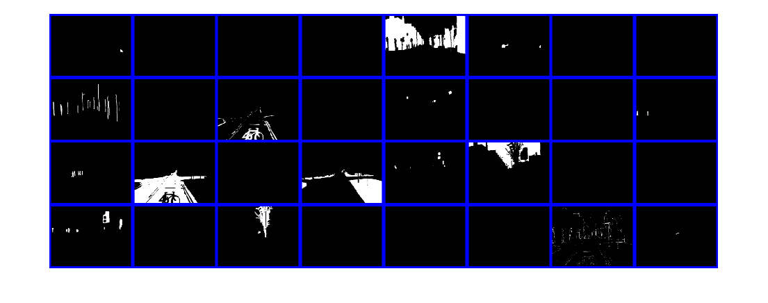

Configure Generator Network

Define a pix2pixHD generator network that generates a scene image from a depth-wise one-hot encoded segmentation map. This input has same height and width as the original segmentation map and the same number of channels as classes.

generatorInputSize = [imageSize numClasses];

Create the pix2pixHD generator network using the pix2pixHDGlobalGenerator (Image Processing Toolbox) function.

dlnetGenerator = pix2pixHDGlobalGenerator(generatorInputSize);

Display the network architecture.

analyzeNetwork(dlnetGenerator)

Note that this example shows the use of pix2pixHD global generator for generating images of size 576-by-768 pixels. To create local enhancer networks that generate images at higher resolution such as 1152-by-1536 pixels or even higher, you can use the addPix2PixHDLocalEnhancer (Image Processing Toolbox) function. The local enhancer networks help generate fine level details at very high resolutions.

Configure Discriminator Network

Define the patch GAN discriminator networks that classifies an input image as either real (1) or fake (0). This example uses two discriminator networks at different input scales, also known as multiscale discriminators. The first scale is the same size as the image size, and the second scale is half the size of image size.

The input to the discriminator is the depth-wise concatenation of the one-hot encoded segmentation maps and the scene image to be classified. Specify the number of channels input to the discriminator as the total number of labeled classes and image color channels.

numImageChannels = 3;
numChannelsDiscriminator = numClasses + numImageChannels;

Specify the input size of the first discriminator. Create the patch GAN discriminator with instance normalization using the patchGANDiscriminator (Image Processing Toolbox) function.

discriminatorInputSizeScale1 = [imageSize numChannelsDiscriminator];
dlnetDiscriminatorScale1 = patchGANDiscriminator(discriminatorInputSizeScale1,NormalizationLayer="instance");

Specify the input size of the second discriminator as half the image size, then create the second patch GAN discriminator.

discriminatorInputSizeScale2 = [floor(imageSize)./2 numChannelsDiscriminator];
dlnetDiscriminatorScale2 = patchGANDiscriminator(discriminatorInputSizeScale2,NormalizationLayer="instance");

Visualize the networks.

analyzeNetwork(dlnetDiscriminatorScale1);
analyzeNetwork(dlnetDiscriminatorScale2);

Define Model Gradients and Loss Functions

The helper function modelGradients calculates the gradients and adversarial loss for the generator and discriminator. The function also calculates the feature matching loss and VGG loss for the generator. This function is defined in Supporting Functions section of this example.

Generator Loss

The objective of the generator is to generate images that the discriminator classifies as real (1). The generator loss consists of three losses.

The adversarial loss is computed as the squared difference between a vector of ones and the discriminator predictions on the generated image. ${Y_{}^{ˆ}}_{g e n e r a t e d}$ are discriminator predictions on the image generated by the generator. This loss is implemented using part of the pix2pixhdAdversarialLoss helper function defined in the Supporting Functions section of this example.

$l o s s A d v e r s a r i a l G e n e r a t o r = (1 - {Y_{}^{ˆ}}_{g e n e r a t e d})^{2}$

The feature matching loss penalises the $L^{1}$ distance between the real and generated feature maps obtained as predictions from the discriminator network. $T$ is total number of discriminator feature layers. $Y_{r e a l}$ and ${Y_{}^{ˆ}}_{g e n e r a t e d}$ are the ground truth images and generated images, respectively. This loss is implemented using the pix2pixhdFeatureMatchingLoss helper function defined in the Supporting Functions section of this example

$l o s s F e a t u r e M a t c h i n g = \sum_{i = 1}^{T} | | Y_{r e a l} - {Y_{}^{ˆ}}_{g e n e r a t e d} | |_{1}$

The perceptual loss penalises the $L^{1}$ distance between real and generated feature maps obtained as predictions from a feature extraction network. $T$ is total number of feature layers. $Y_{V g g R e a l}$ and ${Y_{}^{ˆ}}_{V g g G e n e r a t e d}$ are network predictions for ground truth images and generated images, respectively. This loss is implemented using the pix2pixhdVggLoss helper function defined in the Supporting Functions section of this example. The feature extraction network is created in Load Feature Extraction Network.

$l o s s V g g = \sum_{i = 1}^{T} | | Y_{V g g R e a l} - {Y_{}^{ˆ}}_{V g g G e n e r a t e d} | |_{1}$

The overall generator loss is a weighted sum of all three losses. $λ_{1}$ , $λ_{2}$ , and $λ_{3}$ are the weight factors for adversarial loss, feature matching loss, and perceptual loss, respectively.

$l o s s G e n e r a t o r = λ_{1} * l o s s A d v e r s a r i a l G e n e r a t o r + λ_{2} * l o s s F e a t u r e M a t c h i n g + λ_{3} * l o s s P e r c e p t u a l$

Note that the adversarial loss and feature matching loss for the generator are computed for two different scales.

Discriminator Loss

The objective of the discriminator is to correctly distinguish between ground truth images and generated images. The discriminator loss is a sum of two components:

The squared difference between a vector of ones and the predictions of the discriminator on real images
The squared difference between a vector of zeros and the predictions of the discriminator on generated images

$l o s s D i s c r i m i n a t o r = (1 - Y_{r e a l})^{2} + (0 - {Y_{}^{ˆ}}_{g e n e r a t e d})^{2}$

The discriminator loss is implemented using part of the pix2pixhdAdversarialLoss helper function defined in the Supporting Functions section of this example. Note that adversarial loss for the discriminator is computed for two different discriminator scales.

Load Pretrained Feature Extraction Network

This example modifies a pretrained VGG-19 deep neural network to extract the features of the real and generated images at various layers. These multilayer features are used to compute the perceptual loss of the generator.

Get a pretrained VGG-19 network using the imagePretrainedNetwork function. VGG-19 requires the Deep Learning Toolbox™ Model for VGG-19 Network support package. If this support package is not installed, then the function provides a download link.

netVGG = imagePretrainedNetwork("vgg19");

Configure Feature Extraction Network

Visualize the network architecture using the Deep Network Designer app.

deepNetworkDesigner(netVGG)

To make the VGG-19 network suitable for feature extraction, keep the layers up to "pool5" and remove all of the fully connected layers from the network. The resulting network is a fully convolutional network.

netVGG = dlnetwork(netVGG.Layers(1:38));

Create a new image input layer with no normalization. Replace the original image input layer with the new layer.

inp = imageInputLayer([imageSize 3],Normalization="None",Name="Input");
netVGG = replaceLayer(netVGG,"input",inp);
netVGG = initialize(netVGG);

Train the Network

Specify Training Options

Specify the options for Adam optimization. Train for 60 epochs. Specify identical options for the generator and discriminator networks.

Specify an equal learning rate of 0.0002.
Initialize the trailing average gradient and trailing average gradient-square decay rates with [].
Use a gradient decay factor of 0.5 and a squared gradient decay factor of 0.999.
Use a mini-batch size of 1 for training.

numEpochs = 60;
learningRate = 0.0002;
trailingAvgGenerator = [];
trailingAvgSqGenerator = [];
trailingAvgDiscriminatorScale1 = [];
trailingAvgSqDiscriminatorScale1 = [];
trailingAvgDiscriminatorScale2 = [];
trailingAvgSqDiscriminatorScale2 = [];
gradientDecayFactor = 0.5;
squaredGradientDecayFactor = 0.999;
miniBatchSize = 1;

Create a minibatchqueue object that manages the mini-batching of observations in a custom training loop. The minibatchqueue object also casts data to a dlarray object that enables auto differentiation in deep learning applications.

Specify the mini-batch data extraction format as SSCB (spatial, spatial, channel, batch). Set the DispatchInBackground name-value pair argument as the boolean returned by canUseGPU. If a supported GPU is available for computation, then the minibatchqueue object preprocesses mini-batches in the background in a parallel pool during training.

mbqTrain = minibatchqueue(dsTrain,MiniBatchSiz=miniBatchSize, ...
   MiniBatchFormat="SSCB",DispatchInBackground=canUseGPU);

By default, the example downloads a pretrained version of the pix2pixHD generator network for the CamVid data set by using the helper function downloadTrainedPix2PixHDNet. The helper function is attached to the example as a supporting file. The pretrained network enables you to run the entire example without waiting for training to complete.

To train the network, set the doTraining variable in the following code to true. Train the model in a custom training loop. For each iteration:

Read the data for current mini-batch using the next function.
Evaluate the model gradients using the dlfeval function and the modelGradients helper function.
Update the network parameters using the adamupdate function.
Update the training progress plot for every iteration and display various computed losses.

Train on a GPU if one is available. Using a GPU requires Parallel Computing Toolbox™ and a CUDA® enabled NVIDIA® GPU. For more information, see GPU Computing Requirements (Parallel Computing Toolbox).

Training takes about 22 hours on an NVIDIA™ Titan RTX and can take even longer depending on your GPU hardware. If your GPU device has less memory, try reducing the size of the input images by specifying the imageSize variable as [480 640] in the Prepare Data for Training section of the example.

doTraining = false;
if doTraining
    fig = figure;    
    
    lossPlotter = configureTrainingProgressPlotter(fig);
    iteration = 0;

    % Loop over epochs
    for epoch = 1:numEpochs
        
        % Reset and shuffle the data
        reset(mbqTrain);
        shuffle(mbqTrain);
 
        % Loop over each image
        while hasdata(mbqTrain)
            iteration = iteration + 1;
            
            % Read data from current mini-batch
            [dlInputSegMap,dlRealImage] = next(mbqTrain);
            
            % Evaluate the model gradients and the generator state using
            % dlfeval and the GANLoss function listed at the end of the
            % example
            [gradParamsG,gradParamsDScale1,gradParamsDScale2,lossGGAN,lossGFM,lossGVGG,lossD] = dlfeval( ...
                @modelGradients,dlInputSegMap,dlRealImage,dlnetGenerator,dlnetDiscriminatorScale1,dlnetDiscriminatorScale2,netVGG);
            
            % Update the generator parameters
            [dlnetGenerator,trailingAvgGenerator,trailingAvgSqGenerator] = adamupdate( ...
                dlnetGenerator,gradParamsG, ...
                trailingAvgGenerator,trailingAvgSqGenerator,iteration, ...
                learningRate,gradientDecayFactor,squaredGradientDecayFactor);
            
            % Update the discriminator scale1 parameters
            [dlnetDiscriminatorScale1,trailingAvgDiscriminatorScale1,trailingAvgSqDiscriminatorScale1] = adamupdate( ...
                dlnetDiscriminatorScale1,gradParamsDScale1, ...
                trailingAvgDiscriminatorScale1,trailingAvgSqDiscriminatorScale1,iteration, ...
                learningRate,gradientDecayFactor,squaredGradientDecayFactor);
            
            % Update the discriminator scale2 parameters
            [dlnetDiscriminatorScale2,trailingAvgDiscriminatorScale2,trailingAvgSqDiscriminatorScale2] = adamupdate( ...
                dlnetDiscriminatorScale2,gradParamsDScale2, ...
                trailingAvgDiscriminatorScale2,trailingAvgSqDiscriminatorScale2,iteration, ...
                learningRate,gradientDecayFactor,squaredGradientDecayFactor);
            
            % Plot and display various losses
            lossPlotter = updateTrainingProgressPlotter(lossPlotter,iteration, ...
                epoch,numEpochs,lossD,lossGGAN,lossGFM,lossGVGG);
        end
    end
    save("trainedPix2PixHDNet.mat","dlnetGenerator");
    
else    
    trainedPix2PixHDNet_url = "https://ssd.mathworks.com/supportfiles/vision/data/trainedPix2PixHDv2.zip";
    netDir = fullfile(tempdir,"CamVid");
    downloadTrainedPix2PixHDNet(trainedPix2PixHDNet_url,netDir);
    load(fullfile(netDir,"trainedPix2PixHDv2.mat"));
end

Evaluate Generated Images from Test Data

The performance of this trained pix2pixHD network is limited because the number of CamVid training images is relatively small. Additionally, some images belong to an image sequence and therefore are correlated with other images in the training set. To improve the effectiveness of the Pix2PixHD network, train the network using a different data set that has a larger number of training images without correlation.

Because of the limitations, this pix2pixHD network generates more realistic images for some test images than for others. To demonstrate the difference in results, compare the generated images for the first and third test image. The camera angle of the first test image has an uncommon vantage point that faces more perpendicular to the road than the typical training image. In contrast, the camera angle of the third test image has a typical vantage point that faces along the road and shows two lanes with lane markers. The network has significantly better performance generating a realistic image for the third test image than for the first test image.

Get the first ground truth scene image from the test data. Resize the image using bicubic interpolation.

idxToTest = 1;
gtImage = readimage(imdsTest,idxToTest);
gtImage = imresize(gtImage,imageSize,"bicubic");

Get the corresponding pixel label image from the test data. Resize the pixel label image using nearest neighbor interpolation.

segMap = readimage(pxdsTest,idxToTest);
segMap = imresize(segMap,imageSize,"nearest");

Convert the pixel label image to a multichannel one-hot segmentation map by using the onehotencode function.

segMapOneHot = onehotencode(segMap,3,"single");

Create dlarray objects that inputs data to the generator. If a supported GPU is available for computation, then perform inference on a GPU by converting the data to a gpuArray object.

dlSegMap = dlarray(segMapOneHot,"SSCB"); 
if canUseGPU
    dlSegMap = gpuArray(dlSegMap);
end

Generate a scene image from the generator and one-hot segmentation map using the predict function.

dlGeneratedImage = predict(dlnetGenerator,dlSegMap);
generatedImage = extractdata(gather(dlGeneratedImage));

The final layer of the generator network produces activations in the range [-1, 1]. For display, rescale the activations to the range [0, 1].

generatedImage = rescale(generatedImage);

For display, convert the labels from categorical labels to RGB colors by using the label2rgb (Image Processing Toolbox) function.

coloredSegMap = label2rgb(segMap,cmap);

Display the RGB pixel label image, generated scene image, and ground truth scene image in a montage.

figure
montage({coloredSegMap generatedImage gtImage},Size=[1 3])
title("Test Pixel Label Image " + idxToTest + " with Generated and Ground Truth Scene Images")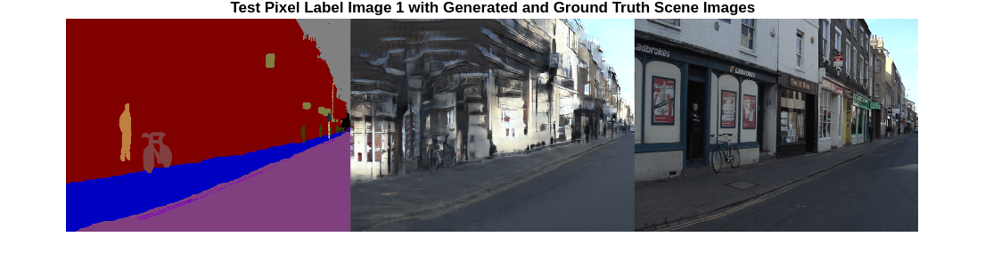

Get the third ground truth scene image from the test data. Resize the image using bicubic interpolation.

idxToTest = 3;  
gtImage = readimage(imdsTest,idxToTest);
gtImage = imresize(gtImage,imageSize,"bicubic");

To get the third pixel label image from the test data and to generate the corresponding scene image, you can use the helper function evaluatePix2PixHD. This helper function is attached to the example as a supporting file.

The evaluatePix2PixHD function performs the same operations as the evaluation of the first test image:

Get a pixel label image from the test data. Resize the pixel label image using nearest neighbor interpolation.
Convert the pixel label image to a multichannel one-hot segmentation map using the onehotencode function.
Create a dlarray object to input data to the generator. For GPU inference, convert the data to a gpuArray object.
Generate a scene image from the generator and one-hot segmentation map using the predict function.
Rescale the activations to the range [0, 1].

[generatedImage,segMap] = evaluatePix2PixHD(pxdsTest,idxToTest,imageSize,dlnetGenerator);

For display, convert the labels from categorical labels to RGB colors by using the label2rgb (Image Processing Toolbox) function.

coloredSegMap = label2rgb(segMap,cmap);

Display the RGB pixel label image, generated scene image, and ground truth scene image in a montage.

figure
montage({coloredSegMap generatedImage gtImage},Size=[1 3])
title("Test Pixel Label Image " + idxToTest + " with Generated and Ground Truth Scene Images")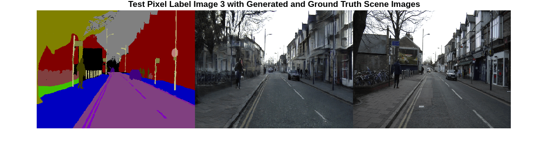

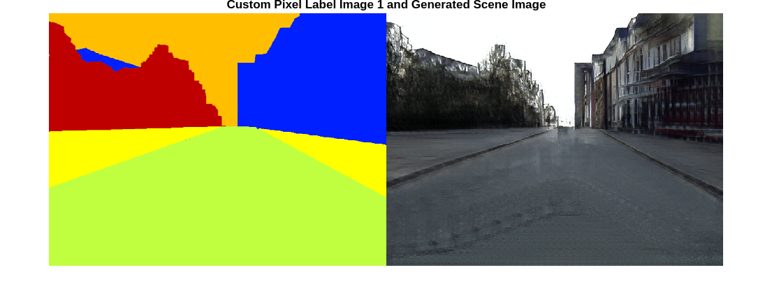
Evaluate Generated Images from Custom Pixel Label Images

To evaluate how well the network generalizes to pixel label images outside the CamVid data set, generate scene images from custom pixel label images. This example uses pixel label images that were created using the Image Labeler (Computer Vision Toolbox) app. The pixel label images are attached to the example as supporting files. No ground truth images are available.

Create a pixel label datastore that reads and processes the pixel label images in the current example directory.

cpxds = pixelLabelDatastore(pwd,classes,labelIDs);

For each pixel label image in the datastore, generate a scene image using the helper function evaluatePix2PixHD.

for idx = 1:length(cpxds.Files)

    % Get the pixel label image and generated scene image
    [generatedImage,segMap] = evaluatePix2PixHD(cpxds,idx,imageSize,dlnetGenerator);
    
    % For display, convert the labels from categorical labels to RGB colors
    coloredSegMap = label2rgb(segMap);
    
    % Display the pixel label image and generated scene image in a montage
    figure
    montage({coloredSegMap generatedImage})
    title("Custom Pixel Label Image " + num2str(idx) + " and Generated Scene Image")

end

Supporting Functions

Model Gradients Function

The modelGradients helper function calculates the gradients and adversarial loss for the generator and discriminator. The function also calculates the feature matching loss and VGG loss for the generator.

function [gradParamsG,gradParamsDScale1,gradParamsDScale2,lossGGAN,lossGFM,lossGVGG,lossD] = modelGradients(inputSegMap,realImage,generator,discriminatorScale1,discriminatorScale2,netVGG)
              
    % Compute the image generated by the generator given the input semantic
    % map.
    generatedImage = forward(generator,inputSegMap);
    
    % Define the loss weights
    lambdaDiscriminator = 1;
    lambdaGenerator = 1;
    lambdaFeatureMatching = 5;
    lambdaVGG = 5;
    
    % Concatenate the image to be classified and the semantic map
    inpDiscriminatorReal = cat(3,inputSegMap,realImage);
    inpDiscriminatorGenerated = cat(3,inputSegMap,generatedImage);
    
    % Compute the adversarial loss for the discriminator and the generator
    % for first scale.
    [DLossScale1,GLossScale1,realPredScale1D,fakePredScale1G] = pix2pixHDAdverserialLoss(inpDiscriminatorReal,inpDiscriminatorGenerated,discriminatorScale1);
    
    % Scale the generated image, the real image, and the input semantic map to
    % half size
    resizedRealImage = dlresize(realImage,Scale=0.5,Method="linear");
    resizedGeneratedImage = dlresize(generatedImage,Scale=0.5,Method="linear");
    resizedinputSegMap = dlresize(inputSegMap,Scale=0.5,Method="nearest");
    
    % Concatenate the image to be classified and the semantic map
    inpDiscriminatorReal = cat(3,resizedinputSegMap,resizedRealImage);
    inpDiscriminatorGenerated = cat(3,resizedinputSegMap,resizedGeneratedImage);
    
    % Compute the adversarial loss for the discriminator and the generator
    % for second scale.
    [DLossScale2,GLossScale2,realPredScale2D,fakePredScale2G] = pix2pixHDAdverserialLoss(inpDiscriminatorReal,inpDiscriminatorGenerated,discriminatorScale2);
    
    % Compute the feature matching loss for first scale.
    FMLossScale1 = pix2pixHDFeatureMatchingLoss(realPredScale1D,fakePredScale1G);
    FMLossScale1 = FMLossScale1 * lambdaFeatureMatching;
    
    % Compute the feature matching loss for second scale.
    FMLossScale2 = pix2pixHDFeatureMatchingLoss(realPredScale2D,fakePredScale2G);
    FMLossScale2 = FMLossScale2 * lambdaFeatureMatching;
    
    % Compute the VGG loss
    VGGLoss = pix2pixHDVGGLoss(realImage,generatedImage,netVGG);
    VGGLoss = VGGLoss * lambdaVGG;
    
    % Compute the combined generator loss
    lossGCombined = GLossScale1 + GLossScale2 + FMLossScale1 + FMLossScale2 + VGGLoss;
    lossGCombined = lossGCombined * lambdaGenerator;
    
    % Compute gradients for the generator
    gradParamsG = dlgradient(lossGCombined,generator.Learnables,RetainData=true);
    
    % Compute the combined discriminator loss
    lossDCombined = (DLossScale1 + DLossScale2)/2 * lambdaDiscriminator;
    
    % Compute gradients for the discriminator scale1
    gradParamsDScale1 = dlgradient(lossDCombined,discriminatorScale1.Learnables,RetainData=true);
    
    % Compute gradients for the discriminator scale2
    gradParamsDScale2 = dlgradient(lossDCombined,discriminatorScale2.Learnables);
    
    % Log the values for displaying later
    lossD = gather(extractdata(lossDCombined));
    lossGGAN = gather(extractdata(GLossScale1 + GLossScale2));
    lossGFM  = gather(extractdata(FMLossScale1 + FMLossScale2));
    lossGVGG = gather(extractdata(VGGLoss));
end

Adversarial Loss Function

The helper function pix2pixHDAdverserialLoss computes the adversarial loss gradients for the generator and the discriminator. The function also returns feature maps of the real image and synthetic images.

function [DLoss,GLoss,realPredFtrsD,genPredFtrsD] = pix2pixHDAdverserialLoss(inpReal,inpGenerated,discriminator)

    % Discriminator layer names containing feature maps
    featureNames = ["act_top","act_mid_1","act_mid_2","act_tail","conv2d_final"];
    
    % Get the feature maps for the real image from the discriminator    
    realPredFtrsD = cell(size(featureNames));
    [realPredFtrsD{:}] = forward(discriminator,inpReal,Outputs=featureNames);
    
    % Get the feature maps for the generated image from the discriminator    
    genPredFtrsD = cell(size(featureNames));
    [genPredFtrsD{:}] = forward(discriminator,inpGenerated,Outputs=featureNames);
    
    % Get the feature map from the final layer to compute the loss
    realPredD = realPredFtrsD{end};
    genPredD = genPredFtrsD{end};
    
    % Compute the discriminator loss
    DLoss = (1 - realPredD).^2 + (genPredD).^2;
    DLoss = mean(DLoss,"all");
    
    % Compute the generator loss
    GLoss = (1 - genPredD).^2;
    GLoss = mean(GLoss,"all");
end

Feature Matching Loss Function

The helper function pix2pixHDFeatureMatchingLoss computes the feature matching loss between a real image and a synthetic image generated by the generator.

function featureMatchingLoss = pix2pixHDFeatureMatchingLoss(realPredFtrs,genPredFtrs)

    % Number of features
    numFtrsMaps = numel(realPredFtrs);
    
    % Initialize the feature matching loss
    featureMatchingLoss = 0;
    
    for i = 1:numFtrsMaps
        % Get the feature maps of the real image
        a = extractdata(realPredFtrs{i});
        % Get the feature maps of the synthetic image
        b = genPredFtrs{i};
        
        % Compute the feature matching loss
        featureMatchingLoss = featureMatchingLoss + mean(abs(a - b),"all");
    end
end

Perceptual VGG Loss Function

The helper function pix2pixHDVGGLoss computes the perceptual VGG loss between a real image and a synthetic image generated by the generator.

function vggLoss = pix2pixHDVGGLoss(realImage,generatedImage,netVGG)

    featureWeights = [1.0/32 1.0/16 1.0/8 1.0/4 1.0];
    
    % Initialize the VGG loss
    vggLoss = 0;
    
    % Specify the names of the layers with desired feature maps
    featureNames = ["relu1_1","relu2_1","relu3_1","relu4_1","relu5_1"];
    
    % Extract the feature maps for the real image
    activReal = cell(size(featureNames));
    [activReal{:}] = forward(netVGG,realImage,Outputs=featureNames);
    
    % Extract the feature maps for the synthetic image
    activGenerated = cell(size(featureNames));
    [activGenerated{:}] = forward(netVGG,generatedImage,Outputs=featureNames);
    
    % Compute the VGG loss
    for i = 1:numel(featureNames)
        vggLoss = vggLoss + featureWeights(i)*mean(abs(activReal{i} - activGenerated{i}),"all");
    end
end

References

[1] Wang, Ting-Chun, Ming-Yu Liu, Jun-Yan Zhu, Andrew Tao, Jan Kautz, and Bryan Catanzaro. "High-Resolution Image Synthesis and Semantic Manipulation with Conditional GANs." In 2018 IEEE/CVF Conference on Computer Vision and Pattern Recognition, 8798–8807, 2018. https://doi.org/10.1109/CVPR.2018.00917.

[2] Brostow, Gabriel J., Julien Fauqueur, and Roberto Cipolla. "Semantic Object Classes in Video: A High-Definition Ground Truth Database." Pattern Recognition Letters. Vol. 30, Issue 2, 2009, pp 88-97.