Hypothesis Testing with Two Samples

Use hypothesis testing to analyze gas prices measured across the state of Massachusetts during two separate months.

Introduction

Hypothesis testing is a common method of drawing inferences about a population based on statistical evidence from a sample. As an example, suppose someone says that at a certain time in the state of Massachusetts, the average price of a gallon of regular unleaded gas was $1.15. How could you determine the truth of the statement? You could try to find prices at every gas station in the state at the time. That approach would be definitive, but it could be time-consuming, costly, or even impossible.

A simpler approach would be to find prices at a small number of randomly selected gas stations around the state, and then compute the sample average.

Sample averages differ from one another due to chance variability in the selection process. Suppose your sample average comes out to be $1.18. Is the $0.03 difference an artifact of random sampling or significant evidence that the average price of a gallon of gas was in fact greater than $1.15? Hypothesis testing is a statistical method for making such decisions.

Load and Visualize Data

Load the gas price data in the file gas.mat. The file contains two random samples of prices for a gallon of gas around the state of Massachusetts in 1993. The first sample, price1, contains 20 random observations around the state on a single day in January. The second sample, price2, contains 20 random observations around the state one month later.

load gas
prices = [price1 price2];

Use a normal probability plot to test the assumption that the samples come from normal distributions.

normplot(prices)

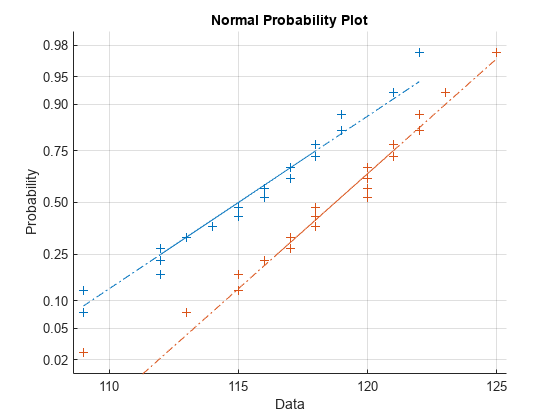
Both sets of points approximately follow straight lines through the first and third quartiles of the samples, indicating approximate normal distributions. The February sample (the right-hand line) shows a slight departure from normality in the lower tail. A shift in the mean from January to February is evident.

Perform Hypothesis Testing

You can use a hypothesis test to quantify the test of normality. Because each sample is relatively small, perform a Lilliefors test.

lillietest(price1)

ans = 
0

lillietest(price2)

ans = 
0

The default significance level of lillietest is 5%. The logical 0 returned by each test indicates a failure to reject the null hypothesis that the samples are normally distributed. This failure might reflect normality in the population, or it might reflect a lack of strong evidence against the null hypothesis due to the small sample size.

Compute the sample means.

sample_means = mean(prices)

sample_means = 1×2

  115.1500  118.5000

Test the null hypothesis that the mean price across the state on the day of the January sample was $1.15. If you know that the standard deviation in prices across the state has historically, and consistently, been $0.04, then a z-test is appropriate. Scale the prices so that they represent dollar amounts instead of cents.

[ztest_h,ztest_p,ztest_ci] = ztest(price1/100,1.15,0.04)

ztest_h = 
0

ztest_p = 
0.8668

ztest_ci = 2×1

    1.1340
    1.1690

The logical output ztest_h is 0, which indicates a failure to reject the null hypothesis at the default significance level of 5%. This result is a consequence of the high probability under the null hypothesis, indicated by the p-value, of observing a value as extreme or more extreme as the z-statistic computed from the sample. The 95% confidence interval on the mean [1.1340,1.1690] includes the hypothesized population mean of $1.15.

Determine whether the later sample offers stronger evidence for rejecting a null hypothesis of a state-wide average price of $1.15 in February. The shift shown in the probability plot and the difference in the computed sample means suggest this result. The shift might indicate a significant fluctuation in the market, raising questions about the validity of using the historical standard deviation. If a known standard deviation cannot be assumed, a t-test is more appropriate.

[ttest_h,ttest_p,ttest_ci] = ttest(price2/100,1.15)

ttest_h = 
1

ttest_p = 
4.9517e-04

ttest_ci = 2×1

    1.1675
    1.2025

The logical output ttest_h is 1, which indicates a rejection of the null hypothesis at the default significance level of 5%. In this case, the 95% confidence interval on the mean does not include the hypothesized population mean of $1.15.

Investigate the shift in prices further. The function ttest2 tests if two independent samples come from normal distributions with unknown and unequal standard deviations and the same mean, against the alternative that the means are unequal.

[ttest2_h,ttest2_p,ttest2_ci] = ttest2(price1,price2,Vartype="unequal")

ttest2_h = 
1

ttest2_p = 
0.0083

ttest2_ci = 2×1

   -5.7846
   -0.9154

The null hypothesis is rejected at the default 5% significance level, and the confidence interval on the difference of means does not include the hypothesized value of 0.

Visualize the shift using notched box plots. The box plots display the distribution of the samples around their medians. The heights of the notches in each box are computed so that the side-by-side boxes have nonoverlapping notches when their medians are different at a default 5% significance level. The computation is based on an assumption of normality in the data, but the comparison is reasonably robust for other distributions. The side-by-side plots provide a kind of visual hypothesis test, comparing medians rather than means.

boxchart(prices,Notch="on")
xticklabels(["January","February"])
xlabel("Month")
ylabel("Prices ($0.01)")
yline([113.4 117.6 117.4 120.6],"--")

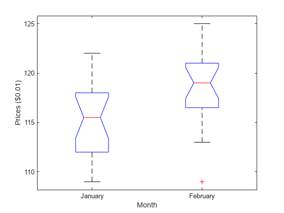
Because the side-by-side boxes have slightly overlapping notches, the plot fails to reject the null hypothesis of equal medians.

Alternatively, you can use the nonparametric Wilcoxon rank sum test to quantify the test of equal medians. The ranksum function tests if two independent samples come from identical continuous (not necessarily normal) distributions with equal medians, against the alternative that they do not have equal medians.

[p,h] = ranksum(price1,price2)

p = 
0.0095

h = logical
   1

The test rejects the null hypothesis of equal medians at the default 5% significance level. This result differs from the previous result using box plots.