다음에 대한 결과:

New in R2022b: GridSizeChangedFcn
tiledlayout() creates a TiledChartLayout object that defines a gridded layout of axes within a figure. When using the 'flow' option, the grid size becomes dynamic and updates as axes are added or as the figure size changes. These features were introduced in R2019b and if you're still stuck on using subplot, you're missing out on several other great features of tiledlayout.
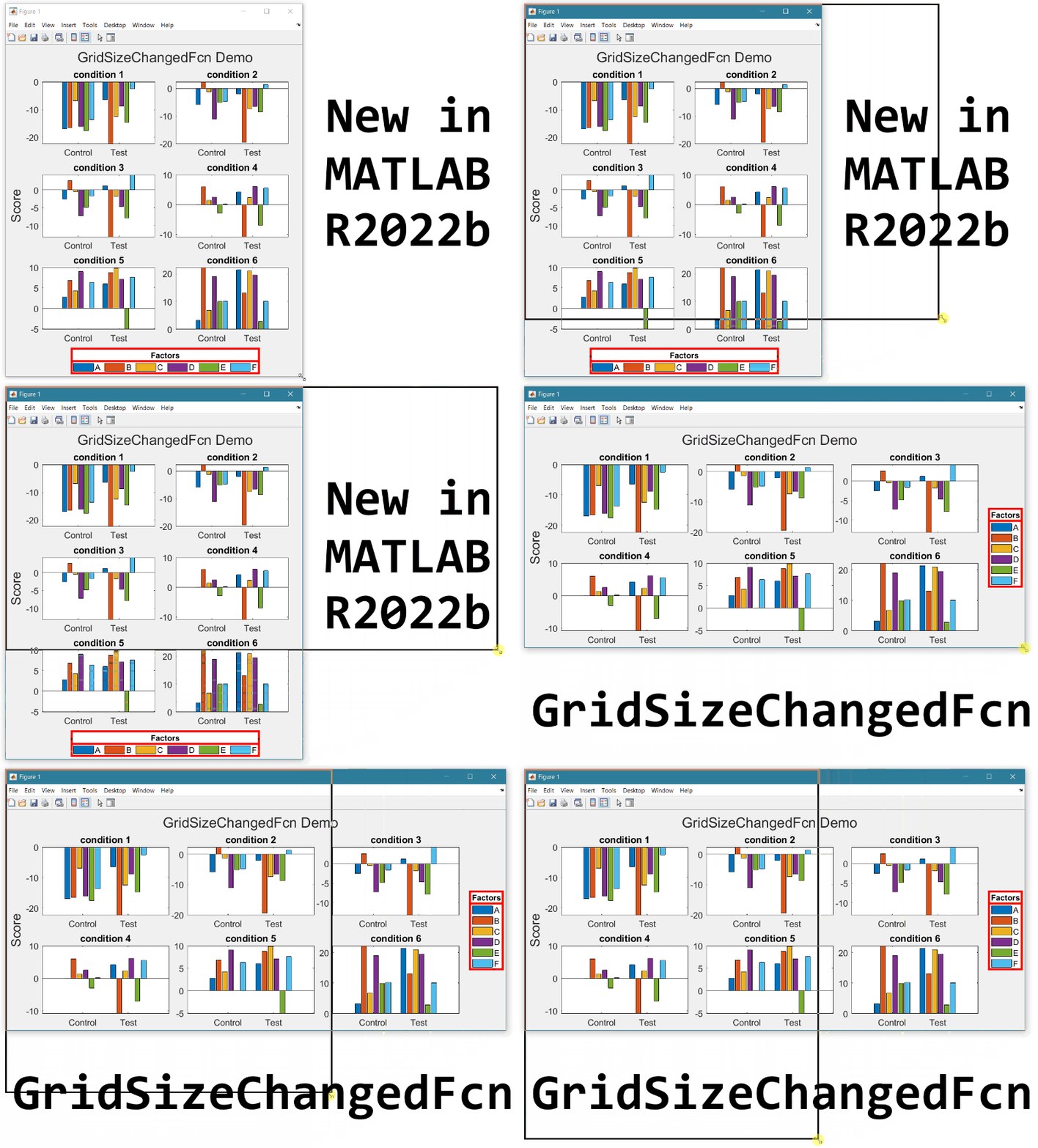
Starting in MATLAB R2022b you can define a callback function that responds to changes to the grid size in flow arrangements by setting the new gridSizeChangedFcn.
Use case
I often use a global legend to represent data across all axes within a figure. When the figure is tall and narrow, I want the legend to be horizontally oriented at the bottom of the figure but when the figure is short and wide, I prefer a vertically oriented legend on the right of the figure. By using the gridSizeChangedFcn, now I can update the legend location and orientation when the grid size changes.
Demo
gridSizeChangeFcn works like all other graphics callback functions. In this demo, I've named the gridSizeChangedFcn "updateLegendLayout", assigned by an anonymous function. The first input is the TiledChartLayout object and the second input is the event object that indicates the old and new grid sizes. The legend handle is also passed into the function. Since all of the tiles contain the same groups of data, the legend is based on data in the last tile.
As long as the legend is valid, the gridSizeChangedFcn updates the location and orientation of the legend so that when the grid is tall, the legend will be horizontal at the bottom of the figure and when the grid is wide, the legend will be vertical at the right of the figure.
Since the new grid size is available as a property in the TiledChartLayout object, I chose not to use the event argument. This way I can directly call the callback function at the end to update the legend without having to create an event.
Run this example from an m-file. Then change the width or height of the figure to demonstrate the legend adjustments.
% Prepare data
data1 = sort(randn(6))*10;
data2 = sort(randn(6))*10;
labels = ["A","B","C","D","E","F"];
groupLabels = categorical(["Control", "Test"]);
% Generate figure
fig = figure;
tcl = tiledlayout(fig, "flow", TileSpacing="compact", Padding="compact");
nTiles = height(data1);
h = gobjects(1,nTiles);
for i = 1:nTiles
ax = nexttile(tcl);
groupedData = [data1(i,:); data2(i,:)];
h = bar(ax,groupLabels, groupedData, "grouped");
title(ax,"condition " + i)
end
title(tcl,"GridSizeChangedFcn Demo")
ylabel(tcl,"Score")
legh = legend(h, labels);
title(legh,"Factors")
% Define and call the GridSizeChangeFcn
tcl.GridSizeChangedFcn = @(tclObj,event)updateLegendLayout(tclObj,event,legh);
updateLegendLayout(tcl,[],legh);
% Manually resize the vertical and horizontal dimensions of the figure
function updateLegendLayout(tclObj,~,legh)
% Evoked when the TiledChartLayout grid size changes in flow arrangements.
% tclObj - TiledChartLayout object
% event - (unused in this demo) contains old and new grid size
% legh - legend handle
if isgraphics(legh,'legend')
if tclObj.GridSize(1) > tclObj.GridSize(2)
legh.Layout.Tile = "south";
legh.Orientation = "horizontal";
else
legh.Layout.Tile = "east";
legh.Orientation = "vertical";
end
end
end
Give it a shot in MATLAB R2022b
- Replace the legend with a colorbar to update the location and orientation of the colorbar.
- Define a GridSizeChangedFcn within the loop so that it is called every time a tile is added.
- Create a figure with many tiles (~20) and dynamically set a color to each row of axes.
- Assign xlabels only to the bottom row of tiles and ylabels to only the left column of tiles.
Learn about other new features
This article is attached as a live script.

Uniform spacing and the problem of round-off error
The vector [3 4 5 6 7 8 9] is uniformly spaced with a step size of 1. So is [3 2 1 0 -1 -2] but with a step size of -1.
The vector [1 2 4 8] is not uniformly spaced.
A vector v with uniform spacing has the same finite interval or step size between consecutive elements of the vector. But sometimes round-off error poses a problem in calculating uniformity.
Take, for example, the vector produced by
format shortg
v = linspace(1,9,7)
v = 1x7
1 2.3333 3.6667 5 6.3333 7.6667 9
Linspace produces linearly spaced vectors but the intervals between elements of v, computed by diff(v), are not identical.
dv = diff(v)
dv = 1x6
1.3333 1.3333 1.3333 1.3333 1.3333 1.3333
dv == dv(1)
ans = 1×6 logical array
1 0 0 1 0 1
diff(dv)
ans = 1x5
4.4409e-16 0 -4.4409e-16 8.8818e-16 -8.8818e-16
Some extra steps are therefore necessary to set a tolerance that ignores error introduced by floating point arithmetic.
New in R2022b: isuniform
Determining uniformity of a vector became a whole lot easier in MATLAB R2022b with the new isuniform function.
isuniform returns a logical scalar indicating whether vector v is uniformly spaced within a round-off tolerance and returns the step size (or NaN if v is not uniform).
Let's look at the results for our vector v,
[tf,step] = isuniform(v)
tf = logical
1
step =
1.3333
How about non-uniformly spaced vector?
[tf,step] = isuniform(logspace(1,5,4))
tf = logical
0
step =
NaN
Give it a shot in MATLAB R2022b
- What happens when all elements of v are equal?
- Can you produce a vector with uniform spacing without using colons or linspace?
- What additional steps would be needed to use isuniform with circular data?
References
- isuniform - documentation
- Floating point numbers - documentation
- Floating point numbers - Cleve's Corner (blog)
This article is attached as a live script.