어서 오세요!
토론은 여러분이 동료를 만나고 더 큰 과제를 함께 해결하며 그 과정에서 즐거움을 찾을 수 있는 공간입니다.
- 최신 업데이트를 보고 싶으신가요? Highlights를 팔로우하세요!
- MATLAB 또는 Simulink 활용 능력을 향상시킬 수 있는 기법을 찾고 계신가요? Tips & Tricks에서 찾을 수 있습니다!
- 수학 관련 농담, 언어유희 또는 밈을 공유하고 싶으신가요? Fun에서 할 수 있습니다!
- 다른 채널이 필요하다고 생각하시나요? Ideas에서 자세히 알려주세요.
업데이트된 토론

What a start! We’ve already seen almost 100 one-button games in Week 1, packed with creative ideas, clever mechanics, and plenty of surprises. Even better, participants have published 18 Tips & Tricks articles sharing how they designed and built their games, what they learned, and how they used agentic AI along the way.
Now for the difficult part: picking the winners. We planned to select 5 Week 1 winners.
We tried. We really did. We ended up picking 12. 😄
And honestly, even 12 doesn’t feel like enough to recognize all the great games we’ve seen.
Congratulations to our Week 1 winners!
Category: Art & Design
Category: Engineering
Category: Anxiety Raising
Category: Sports
Category: Score = 9999
Category: Simple but fun
Category: Humorous
Category: Retro Design
Special Category for Week 2 & Week 3: STEM Education
For Weeks 2 and 3, we’re introducing a special STEM Education category. Our challenge: Can you help someone learn while they’re having fun?
Your game could teach a MATLAB function or programming concept, demonstrate gravity or projectile motion, simulate a scientific experiment, or visualize an engineering concept.
The possibilities are wide open. Just remember: learning + playing = the goal.
And there’s a special prize too: STEM Education winners will receive a MathWorks Stainless Steel Coffee Mug! ☕

If you had to catch up with a spacecraft ahead of you in the same orbit, what would you do?
The intuition is to speed up and catch the spacecraft ahead. In orbit, that’s wrong. To catch something ahead of you, you burn retrograde and slow down.
Why burning retrograde works
Slowing down drops you into a lower orbit. A lower orbit is shorter and faster, so you complete each revolution sooner and gain on the spacecraft ahead every lap.
At the lowest point of that new orbit you’re actually moving faster than your target. Speeding up does the opposite: you climb higher, your orbit takes longer, and you fall behind.
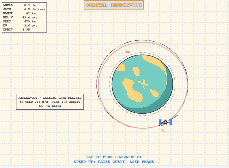
You start in the same 800 km circular orbit as a space station, trailing it by 25–55° with 400 m/s of Δv. One tap starts a burn and the next tap cuts the engine.
Burns alternate automatically: the first is retrograde, the second prograde, then retrograde again, and so on.
How to win
- Win: get within 200 km of the station with a relative speed below 50 m/s.
- Don’t burn up: if your orbit drops below 120 km altitude, you burn up in the atmosphere.
- Watch your fuel: you have 600 m/s of Δv.
- Beat the clock: you have 20 orbits to dock.
Key terms
- Prograde: thrusting along your direction of travel. Speeds you up and raises the opposite side of your orbit.
- Retrograde: thrusting against your direction of travel. Slows you down and lowers the opposite side of your orbit.
- Perigee: the lowest point of an orbit.
- Apogee: the highest point of an orbit.
What I learned building the game: realism vs. playability
I started out trying to make everything 1:1 with real orbital mechanics. It was physically accurate, but it was frustrating to play. Some trade-offs had to be made:
What I kept real
- The game simulates planar Keplerian dynamics. Burns are applied either along (prograde) or against (retrograde) your velocity vector.
- Orbital mechanics: to catch a station that’s ahead of you, you slow down. A retrograde burn reduces your semi-major axis a, and since the orbital period is T = 2π·sqrt(a³/μ), a smaller orbit has a shorter period. You gain on the station every revolution.
- The vis-viva equation v² = μ(2/r − 1/a), shows that speed is highest at periapsis and lowest at apoapsis. At the periapsis of your lower orbit you’re moving faster than the station, even though you got there by braking.
- To stop drifting, do a prograde burn back at the point where you first burned, which is now your apoapsis. Raising a back to the station’s radius recircularises your orbit and matches its period.
What I changed for playability
- Time warping. A real orbit at this altitude takes about 100 minutes. In the game it takes 8 seconds, roughly 750x real time.
- Burn in slow motion. Time runs 4x slower while the engine fires, so you can actually control how long a burn lasts with one button.
- A strong engine. Thrust is about 0.4 m/s², which is way higher than a normal spacecraft but it means a burn takes a few seconds instead of minutes.
- Exaggerated distance. In the game the distance from the station’s orbit is stretched 3x, otherwise the difference of the orbits wouldn't be visible.
- A generous docking gate. A realistic range (tens of km and relative velocity around 15 m/s) was nearly impossible to hit, so I widened it to 200 km and 50 m/s.

In a cath lab, the most important button is a pedal: press it and you see, release it and the image freezes. Every second you press costs radiation dose. That felt like the perfect one-button game.
My entry, X-Ray Guided, simulates a coronary stenting procedure from the groin to the heart. I work on fluoroscopic image quality as a medical physicist, so I wanted the X-ray image and the dose to behave like the real thing, at least where it matters for the game.
How to play
You are on shift in the cath lab. Patients arrive one after another, each with two random traits (obese, tortuous iliacs, tachycardic, small vessel, renal failure, calcified vessel) that change how the case plays. Three complications end your shift.
Each patient has four steps, and the line at the bottom of the screen always tells you what the tap does right now:
- Wire: tap to start pushing the guidewire blind and watch the FEEL bar. When you meet resistance, you can keep pushing blind (risky) or tap to switch fluoroscopy on. With X-rays on, the wire tip rotates: tap when it lines up with the vessel, or wait and let it creep through slowly while the dose climbs.
- Angiography: tap to inject contrast, then tap again at peak opacification to save the reference image of the lesion.
- Stent: without contrast the vessel is invisible. The stent slides along the wire; use the reference image (top left) and the small contrast puffs at each end of its travel, then tap to deploy it on the lesion.
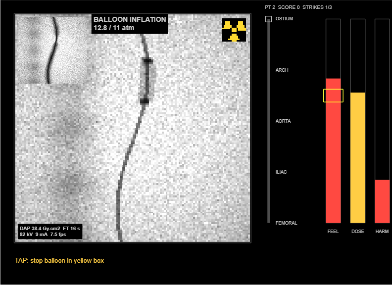
- Balloon: it inflates by itself, faster and faster. Tap inside the yellow box, at nominal pressure.
A full HARM bar, a full DOSE bar, a missed lesion or a wrong inflation is a complication. Score depends on lesion coverage and expansion, minus dose, vessel trauma and time; consecutive clean cases give a multiplier.
One pedal, many jobs
The contest gives you a single tap, with no hold and no release. That turned out to fit the cath lab surprisingly well, because a real procedure is also a sequence of single, well-timed decisions, and each phase asks a different one:
- Navigation: do I need to look? The wire goes up mostly by feel. The tap is the moment you decide that the resistance in your hand is worth some radiation to understand.
- Fluoroscopy on an obstacle: now, or wait? Tapping when the tip lines up is fast but risky; waiting lets the wire creep through safely, and the DOSE bar shows what that patience costs.
- Angiography: when is the vessel best filled? Saving the reference too early or too late leaves you with a poor map of the lesion for the next step.
- Stent: is it on the lesion? With the contrast gone, you deploy from memory of the reference image and from the short puffs, each of which costs extra dose.
- Balloon: when do I stop? Too little and the stent is under-expanded, too much and you overstretch or rupture the vessel.
So the tap always means “act now”, but what it acts on changes with the phase. Two things made this readable: the game moves things by itself (the tip rotates, the stent slides, the balloon inflates), so when you tap is the decision, and not tapping is a decision too; and a line at the bottom of the screen always says what the tap will do next.Real vs. playable
What I kept real
- Most of the wire’s journey is done without X-rays, by feel. Fluoroscopy is switched on when you need it.
- The image is built like a fluoroscopy frame: attenuation of anatomy, vessel and devices, quantum noise that grows with the signal, and a recursive temporal filter that reduces noise but leaves lag behind moving objects. Release the pedal and you are left with the last image hold.
- Cine costs much more than fluoroscopy. Here it is 5 times per second, so the contrast injection and each puff are visible jumps on the DOSE bar.
- Coronary arteries are invisible without contrast, while the stent’s marker bands are not. That is why a good reference image matters.
- An obese patient means a noisier image and more dose for the same procedure.
What I changed for playability
- Time is compressed: a procedure lasts a couple of minutes, so the DAP values on screen are game numbers, and the per-patient limit is a game rule, not a clinical threshold.
- The contrast puffs during stent positioning are automatic, at each end of the stent’s travel, instead of being a separate action.
- The stent and the balloon move by themselves, so that the single tap becomes a timing decision.
- One projection, simplified anatomy, and a vessel that bends only where the obstacles are.
On the code side, the whole X-ray monitor is a single 128x128 image whose CData is rebuilt every frame from an attenuation map, with noise and temporal filtering added in two lines. For fitting everything into the character limit, Ahmed’s post on how the validator counts reformatted code says it better than I could.
How long does your shift last? And if you work in a cath lab: what would you add?

What happens when you take a classic Pac-Man style maze game and limit the player to just one button?
That was the idea behind MAZE FRENZY, my entry for the MATLAB One Button Game Mini Hack.
The player moves automatically through a maze, collecting pellets while avoiding four pursuing ghosts. A single click changes direction at available turns. Power orbs temporarily reverse the chase, allowing players to capture ghosts and earn bonus points.
How to play
- Collect pellets for 10 points each.
- Collect power orbs for 50 points.
- Capture powered up ghosts for 200 points.
- Survive with three lives.
- Clear the maze to advance to faster levels.
Gameplay screenshot
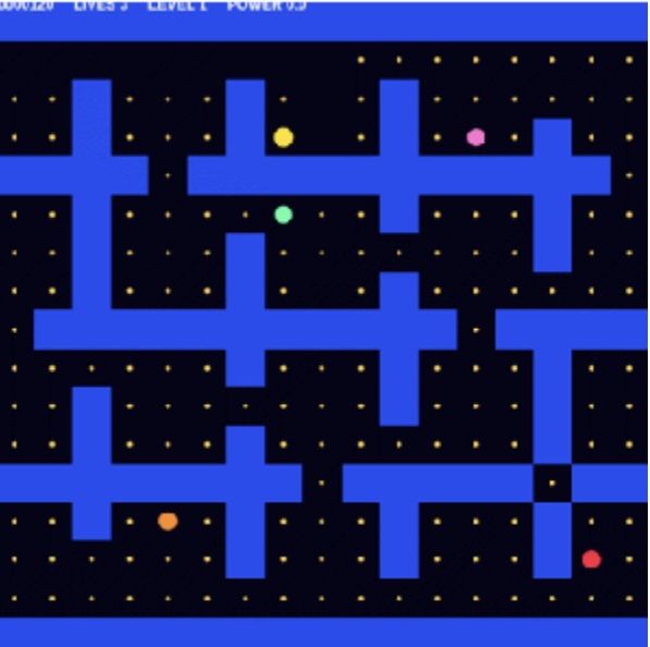
Figure1. Maze gameplay showing the player, ghosts, pellets,
power orbs, and scoreboard.
Inside the MATLAB code
The game follows the init,update, and render architecture.
- init constructs the maze and initializes graphics.
- update handles movement, collisions, scoring, and ghost behavior.
- render updates the existing graphics objects.
The maze uses a logical matrix (true for walls and false for paths). MATLAB functions such as image, scatter, text, find, set, abs, and sprintf handle the graphics and game logic. Ghosts use Manhattan distance calculations to pursue the player and retreat when a power orb is active.
What I'd improve next
I would like to explore breadth first search for smarter ghost navigation, individual ghost personalities, procedural maze layouts, and smoother character animation.
The interesting challenge was making a familiar arcade game work with just one button. It turns movement into a strategic excercise in timing and anticipating the next junction.
How would you approach ghost AI in MATLAB for shortest path search or individual enemy behaviors?

The MATLAB One-Button Game Mini Hack runs from November 2nd through November 29th, 2026! The challenge is to make a game that can be played with one button. I thought this would be a good opportunity to share some of the graphics and programming ideas behind Arcade, a collection of 15 games I developed in MATLAB using Claude Code and the MATLAB MCP Server.
Before the 2024 MATLAB Shorts Mini Hack, Tim Marston published his walkthrough of Little Nemo's airship. I learned a lot from Tim's article, and it inspired me to enter the contest. I hope that sharing some of what goes into these games might encourage a few more people to give it a try this time around as well.
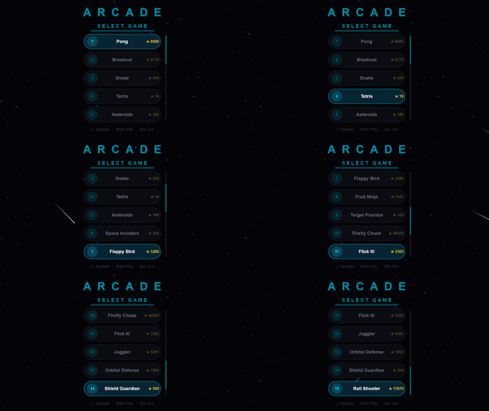
You can download Arcade from File Exchange or GitHub, add the project folder to the MATLAB search path, and run:
Arcade();
Creating and updating graphics
Arcade sports neon-styled graphics. This is accomplished by layering ordinary MATLAB graphics against a dark background. The bright colors used come from the shared GameBase palette, which enables the different games to keep a consistent appearance and accounts for quite a bit of that look.
In Pong, the ball is made by drawing a colored dot, a semitransparent scatter marker and a smaller white dot at the same position. The ball and trail change from cyan through green, gold and red as the ball speeds up, while the center stays white. Against the dark background, these simple shapes give us the bright center and surrounding glow.
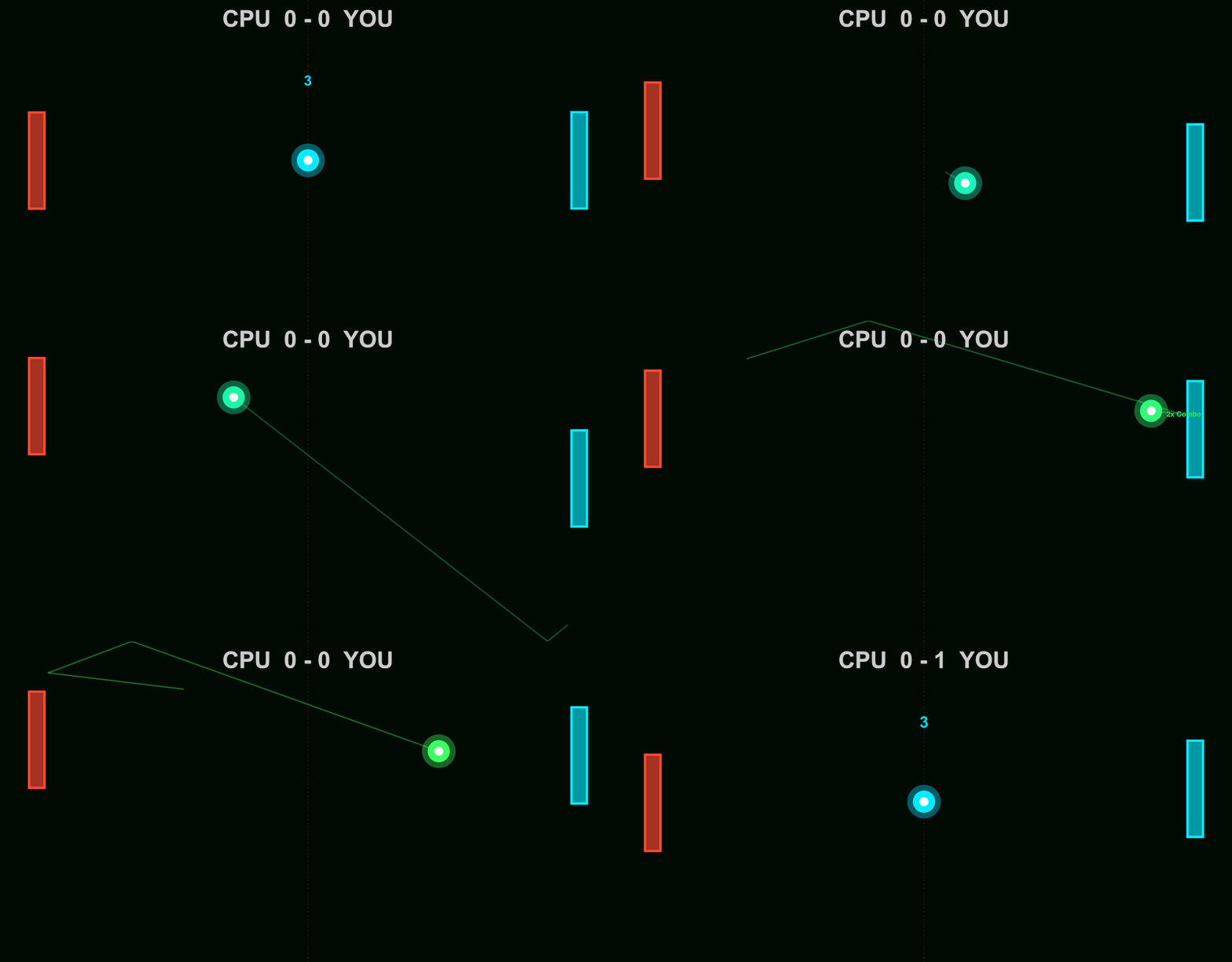
arcadeBallDemo();
worldSize = [854, 480];
position = worldSize / 2;
cyan = [0, 0.92, 1];
radiusParameter = max(3, round(min(worldSize) * 0.035));
baseCoreSize = 2 * radiusParameter;
baseDotSize = 5 * radiusParameter;
baseGlowArea = pi * (1.25 * radiusParameter)^2;
coloredDot = line(ax, NaN, NaN, ...
Marker=".", MarkerSize=baseDotSize, LineStyle="none", Color=[cyan, 0.15]);
glow = scatter(ax, position(1), position(2), baseGlowArea, cyan, "filled", ...
MarkerFaceAlpha=0.4);
core = line(ax, position(1), position(2), ...
Marker=".", MarkerSize=baseCoreSize, LineStyle="none", Color=[1, 1, 1, 1]);
ballLayers = {coloredDot, glow, core};
Here's how the ball looks as each layer is added:

Setting NextPlot="add" preserves the existing graphics as we add the layers. Specifying the axes limits by using XLim and YLim keeps the view in place as the ball moves.
Each drawing call returns a handle to its object. With those handles stored in ballLayers, moving the ball involves assigning its new position to the existing objects:
for layerIndex = 1:numel(ballLayers)
ballLayers{layerIndex}.XData = position(1);
ballLayers{layerIndex}.YData = position(2);
end
drawnow
MathWorks' graphics-performance guidance recommends retaining graphics and updating the properties that change. Pong also checks whether its scores have changed before assigning new score text. Its trail uses preallocated position buffers, wrapping around as new positions arrive, and two retained lines display that history as a broad dim stroke with a narrower bright stroke.
Handling inputs using callback functions
The ball example responds to mouse presses through a callback function. After creating the scene, it assigns a function handle to the figure's WindowButtonDownFcn callback property:
fig.WindowButtonDownFcn = @reverseVerticalDirection;
MATLAB executes the callback function when a mouse button is pressed in the window. In the example, it is nested inside the local animateBall function:
function reverseVerticalDirection(~, ~)
velocity(2) = -velocity(2);
end
The two arguments supplied by MATLAB are the source object and event data. The ~ placeholders indicate that this function doesn't use them. As a nested function, it can access velocity in the enclosing function. Each mouse press reverses the shared vertical velocity, which the next loop iteration uses to move the ball.
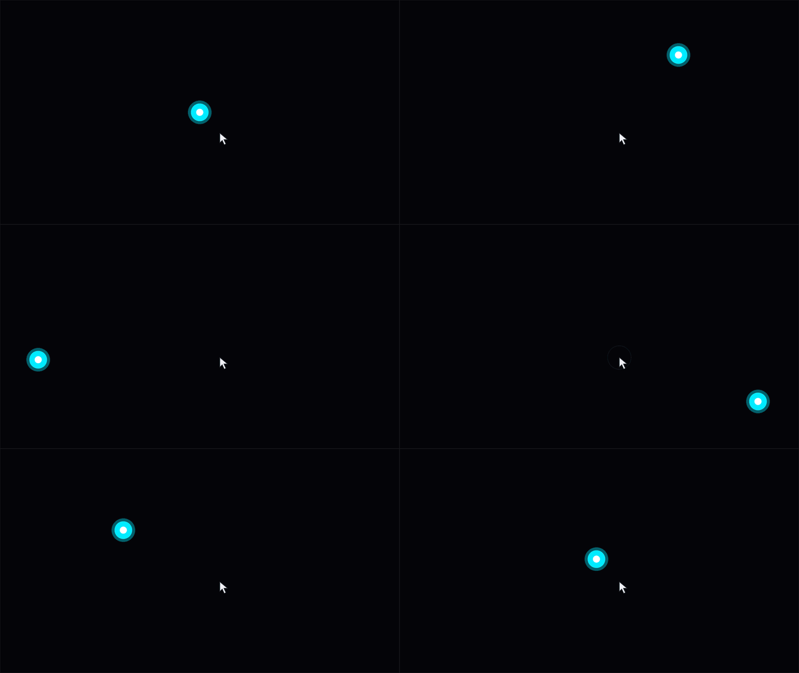
Arcade routes input through methods on the launcher. Its figure's KeyPressFcn callback property is assigned as follows, where obj is the launcher instance:
obj.Fig.KeyPressFcn = @(~, event) obj.onKeyPress(event);
The anonymous function forwards the event data to onKeyPress, where its Key property identifies the key. The launcher handles its own controls and passes appropriate input to the active game. Button release and scrolling have their own callback functions.
Mouse movement can control a paddle or aim a shot. To track the pointer as it moves within the figure, Arcade assigns a callback function to WindowButtonMotionFcn:
obj.Fig.WindowButtonMotionFcn = @(~, ~) obj.onMouseMove();
function onMouseMove(obj)
pointer = obj.Ax.CurrentPoint;
obj.MousePos = pointer(1, 1:2);
end
The axes' CurrentPoint gives the pointer position in game coordinates. MATLAB accounts for the axes' position and size, so the same code works when the playfield is resized or surrounded by margins.
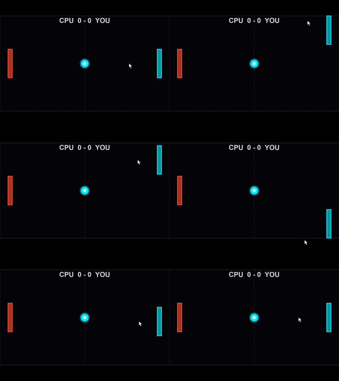
On each game update, the launcher passes the stored position to the active game's onUpdate method. In Pong, obj now refers to the game instance. Once the incoming pos is available, its vertical coordinate determines the player's paddle position:
yLimits = obj.DisplayRange.Y;
if ~any(isnan(pos))
obj.PlayerPaddleY = max(yLimits(1) + obj.PaddleHalfH, ...
min(yLimits(2) - obj.PaddleHalfH, pos(2)));
end
The min and max calls keep the paddle's center at least half a paddle height from either edge. Moving the pointer into a margin therefore leaves the whole paddle inside the playfield. The graphics update then applies that position to the existing paddle patches.
The animation loop's drawnow displays pending graphics changes and processes pending callbacks. Keeping callback functions short allows control to return to the loop promptly.
Animating visual effects
When the orb is launched in Flick It!, a call to spawnHitEffect creates a ring and rays that expand and fade. The launcher advances these shared effects alongside the active game.
In arcadeEffectsDemo.m, each click creates a burst at the mouse position, allowing several bursts to expand and fade together. To try it out, download the function, add its folder to the MATLAB path, and run:
arcadeEffectsDemo();
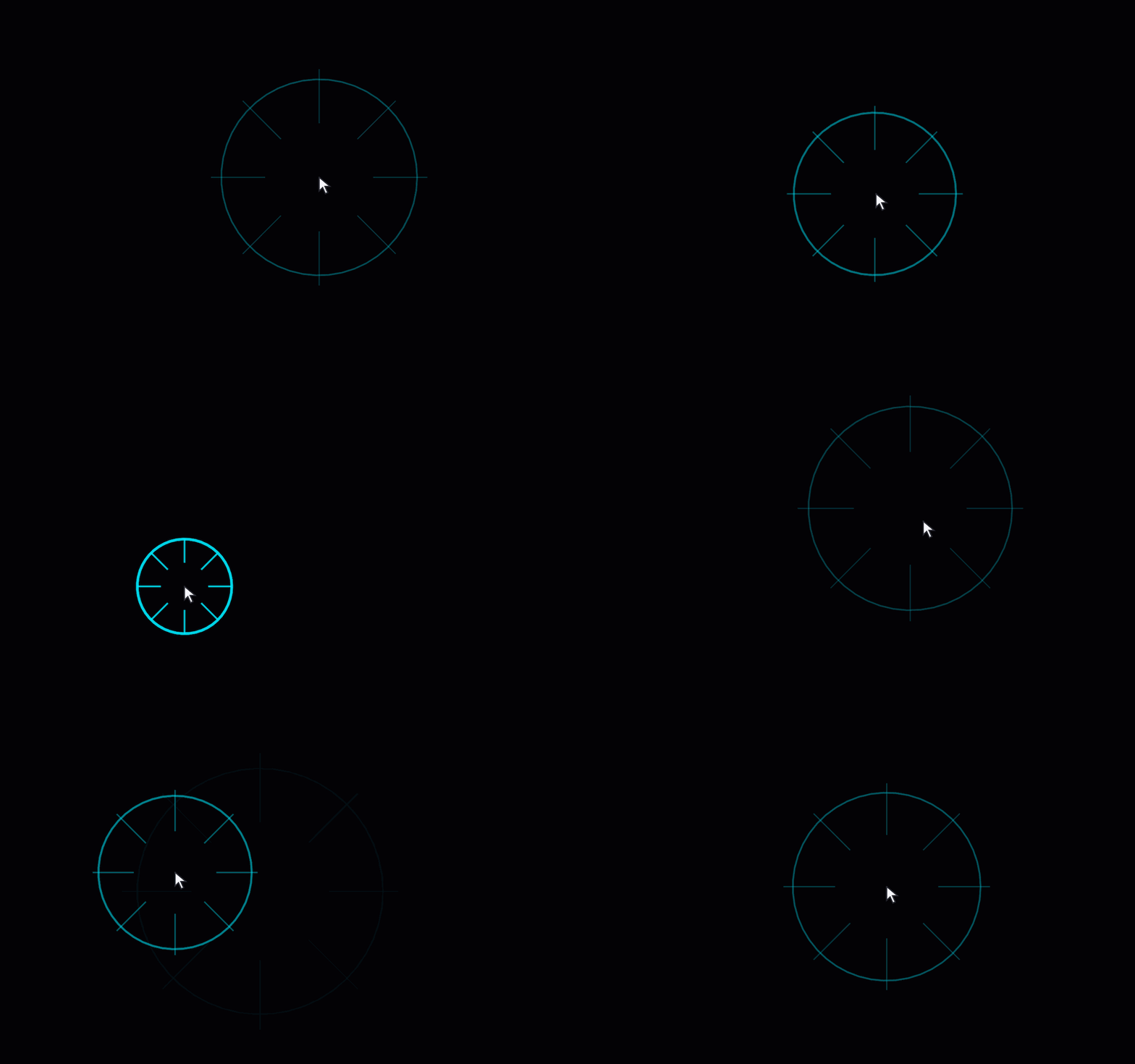
The nested callback function combines mouse-press handling with the mouse-position tracking introduced earlier. Here's the part that creates and stores a new burst:
fig.WindowButtonDownFcn = @createManualImpact;
function createManualImpact(~, ~)
point = ax.CurrentPoint;
position = point(1, 1:2);
if any(~isfinite(position)) || any(position < 0 | position > worldSize)
return
end
[newRing, newRays] = createEffect(position);
activeEffects(end+1) = struct('Ring', newRing, 'Rays', newRays, ...
'Center', position, 'AgeSeconds', 0, 'LastTime', toc(animationClock));
end
The bounds check ignores clicks outside the playfield. createEffect creates the lines, and activeEffects stores their handles, center and timing state. The animation loop updates each burst independently, allowing further clicks while earlier bursts are still expanding.
We can drive the geometry, transparency and line width from a common progress value: 0 when the burst begins and 1 at the end of its lifetime. Inside the function, the ring is updated as follows:
progress = ageSeconds / lifetimeSeconds;
eased = 1 - (1-progress)^2;
opacity = max(0, 1-1.5*eased);
ringRadius = radiusParameter * (1+2.5*eased);
ring.XData = center(1) + ringRadius*ringCos;
ring.YData = center(2) + ringRadius*ringSin;
ring.Color = [cyan, 0.8 * opacity];
ring.LineWidth = max(0.5, 3*(1-eased));
The ease-out expression starts the expansion quickly and slows it down toward the end. The burst fades out before its nominal lifetime finishes. ringCos and ringSin hold the circle's fixed directions, calculated before the loop. Arcade controls the transparency of these lines by assigning an RGBA value to Color, with alpha as the fourth component, ranging from 0 (clear) to 1 (fully opaque).
The row vectors rayCos and raySin contain the eight ray directions. Each ray joins the inner and outer radii, which increase as the burst expands:
innerRadius = radiusParameter * (0.5+1.5*eased);
outerRadius = radiusParameter * (1+3*eased);
for rayIndex = 1:numel(rays)
rays(rayIndex).XData = center(1) + [innerRadius, outerRadius]*rayCos(rayIndex);
rays(rayIndex).YData = center(2) + [innerRadius, outerRadius]*raySin(rayIndex);
rays(rayIndex).Color = [cyan, 0.6 * opacity];
rays(rayIndex).LineWidth = max(0.5, 2*(1-eased));
end
The lines are created when the burst begins, updated throughout its lifetime and deleted when it expires.
Display scaling: Keeping the scene in proportion
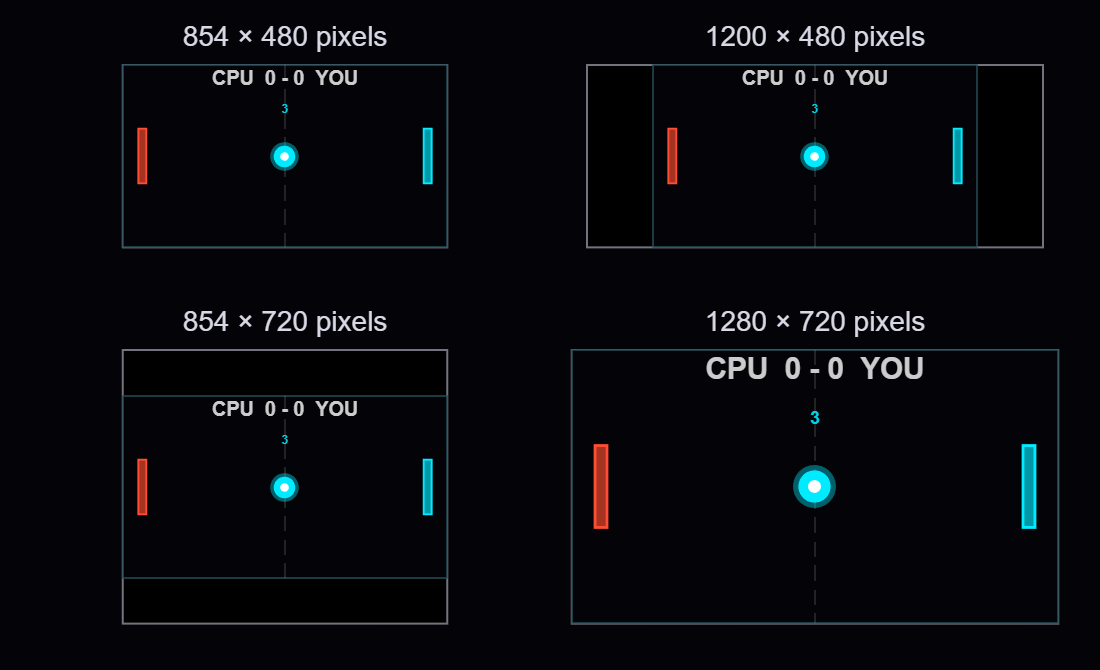
Try making the ball example's window wider while keeping its height the same. Space appears beside the playfield, and the ball still travels between the same boundaries. The example's reference window is 854 by 480 pixels, matching worldSize numerically. Resizing scales the playfield on the screen while the game's coordinate system remains unchanged.
The figure and axes use Units="pixels". Taking the min of the width and height ratios relative to the reference window gives the largest scale factor that fits in both directions. Applying that same scale to both dimensions preserves the playfield's 16:9 aspect ratio.
For a 1200-by-480 window, the height limits the scale to 1. The fitted area remains 854 by 480, leaving (1200-854)/2 = 173 pixels on each side. In a 1280-by-720 window, the playfield grows to approximately 1.5 times its reference width and height. Here are four window sizes at a common page scale:
MATLAB already scales graphics defined in data coordinates as the axes resize. For example, a paddle drawn with patch grows with the axes. In the example, marker sizes, font sizes and line widths use points, while scatter sizes use points squared.

To make a circle twice as wide, we need four times its area. Doubling SizeData multiplies its width by only √2:
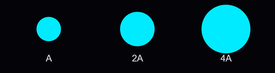
fig.SizeChangedFcn = @fitScene;
The nested fitScene callback function combines the axes calculation with these size updates:
function fitScene(~, ~)
if ~isgraphics(ax)
return
end
availableSize = max(fig.Position(3:4), [1, 1]);
displayScale = min(availableSize ./ worldSize);
fittedSize = worldSize * displayScale;
ax.Position = [(availableSize - fittedSize)/2 + 1, fittedSize];
% Always derive sizes from their reference values
core.MarkerSize = baseCoreSize * displayScale;
coloredDot.MarkerSize = baseDotSize * displayScale;
glow.SizeData = baseGlowArea * displayScale^2;
instruction.FontSize = baseFontSize * displayScale;
playfield.LineWidth = 0.5 * displayScale;
end
The first two entries of ax.Position set the left and bottom position, splitting the unused space equally between opposite sides. The last two give the fitted width and height. The axes limits remain unchanged, so movement and collision calculations keep using the same game coordinates.
At scale 1.5, the marker sizes are multiplied by 1.5 and the scatter area by 2.25. The updated sizes are calculated from their stored reference values. A 34-point reference marker becomes 51 points at scale 1.5, then 68 points at scale 2.
You can also use Units="normalized" to size and position the axes relative to the figure. Arcade's axes setup uses [0 0 1 1] to allocate the full available area:
obj.Ax = axes(obj.Fig, "Units", "normalized", "Position", [0 0 1 1]);
obj.Ax.XLim = obj.DisplayRange.X;
obj.Ax.YLim = obj.DisplayRange.Y;
Arcade's resize method obtains the available dimensions in pixels with getpixelposition and calculates the same display scale. It uses pbaspect to preserve the playfield's aspect ratio. MATLAB fits the playfield within the available space, leaving margins where needed:
axPx = getpixelposition(obj.Ax);
newPs = min(axPx(3) / 854, axPx(4) / 480);
gameAR = diff(obj.DisplayRange.X) / diff(obj.DisplayRange.Y);
pbaspect(obj.Ax, [gameAR 1 1]);
For Arcade, I also wanted markers, text and line widths to grow proportionally with the playfield. MATLAB also supports automatic resizing for text through FontUnits="normalized", which expresses font size as a fraction of the axes plot box height. This works well for text in a playfield with a fixed aspect ratio. Arcade's shared resize helper modifies current property values, using the ratio of the new scale to the previous scale; for example, moving from 51 to 68 points requires multiplying by 2/1.5. The function applies a common display scale to text, markers and line widths, in order to preserve their relative sizes as the window is resized.
FPS scaling: Let elapsed time determine the motion
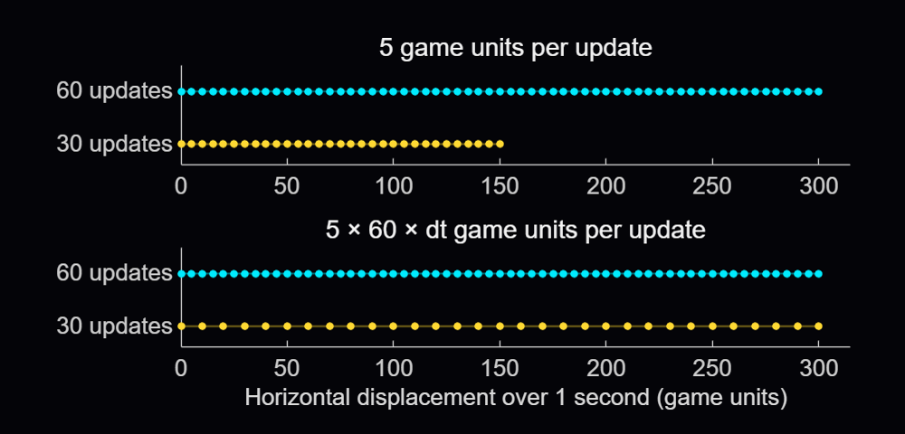
Suppose that the ball moves 5 game units on each update. At 60 updates per second it travels 300 units in a second, but at 30 it travels only 150. Calculating the state, drawing and processing input all contribute to the time between updates, so we need to measure that interval to maintain a consistent speed.
Gianluca Carnielli discusses the relationship between time and animation frames in Animating Science: Creating Time-Sensitive Animations with MATLAB. In his example, he explains how to create a frame-based animation from time-based coordinates, by choosing the video’s duration and frame rate, calculating the simulation timestep between two consecutive frames, and resampling the coordinates using retime.
In a live game, we process player actions and calculate each new state using the time elapsed since the previous update. Arcade expresses many motion parameters per reference interval, using 60 frames per second (FPS) as its reference frequency. An elapsed time of 1/60 seconds represents 1 reference interval, while 1/30 seconds represents 2. In the example, we define the velocity and reference frequency before the loop and start the clock with tic once the initial scene is displayed:
velocity = [5, 3]; % Game units per reference interval
referenceFPS = 60; % Reference intervals per second
animationClock = tic;
previousTime = 0;
currentTime = toc(animationClock);
dtSeconds = min(currentTime - previousTime, 0.1);
previousTime = currentTime;
dtScale = dtSeconds * referenceFPS;
position = position + velocity * dtScale;
Here dtSeconds is in seconds, and dtScale counts reference intervals. A horizontal velocity of 5 now gives a movement of 10 game units over 1/30 second. Taking 30 steps of 10 units covers the same 300 units as 60 steps of 5 units. The samples are farther apart, so the motion can look less smooth:
The min(..., 0.1) caps a single represented interval at 0.1 seconds (10 FPS) to limit jumps after a stall. If an update arrives after 0.5 seconds, the code advances only 0.1 seconds, and the remaining 0.4 seconds are discarded.
The reference frequency is 60 FPS; the actual update rate depends on execution. We could also use game units per second and write position = position + velocityPerSecond * dtSeconds.
Arcade schedules its updates with a timer. The callback function assigned to its TimerFcn property calls the launcher's frame-update method:
obj.RenderTimer = timer(ExecutionMode="fixedSpacing", ...
Period=0.02, TimerFcn=@(~, ~) obj.onFrame());
start(obj.RenderTimer)
With fixedSpacing, the period begins after the preceding callback function finishes. The function's own work therefore contributes to the interval between updates. The launcher measures the full interval and passes the resulting time scale to the active game.
arcadeBallDemo(Inf, 0.04);
Its measured interval includes both the pause and the surrounding work. Both Arcade and the example use the full drawnow command. The limitrate option can reduce rendering work by limiting display updates to 20 per second; its suitability depends on the animation's required display rate.
Flick It! multiplies its velocity by friction^dtScale, where friction is the fraction of velocity retained over one reference interval. Over 2 intervals, the multiplier is the square of that factor, equivalent to applying it once in each interval. This makes the velocity decay follow the elapsed time.
For accelerating objects, the numerical approximation can still change with step size, and collisions need to account for movement between samples. Pong checks when the ball crosses the paddle's front face and interpolates its vertical position there, allowing a contact to be detected between two displayed positions.
Organizing games using classes
Arcade's registry stores a constructor function handle for each game. When a game is selected, the launcher calls the corresponding constructor to instantiate the game class. Here's an adaptation of the launch sequence, with Pong selected explicitly and obj referring to the launcher:
createGame = @games.Pong;
game = createGame();
game.FontScale = obj.FontScale;
game.init(obj.Ax, obj.DisplayRange)
game.beginGame()
obj.ActiveGame = game;
Each game subclasses engine.GameBase. The shared init method sets up the session and calls the game's onInit, which creates its state and graphics. Assigning FontScale beforehand lets newly created markers and text use the current display size. The launcher stops its render timer before creating the game and restarts it after the initialized game is assigned to ActiveGame. This prevents timer callbacks from running while the game’s state and graphics are being created.
GameBase declares four abstract methods that each game class must implement:
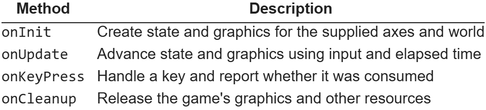
The launcher calls onUpdate on its active game, and MATLAB dispatches that call to the selected subclass. Pong implements paddle and ball movement; Flappy Bird advances its bird and pipes. All games inherit methods for scoring, combo handling and visual effects from GameBase. Window management, menus, timing and common services stay with the launcher.
As a handle class, GameBase lets the launcher keep a reference to the same game instance while its state changes. Position arrays, velocities, scores and graphics handles belong to that instance. Property access attributes allow the host to read the common score while leaving changes under the control of the game classes.
Flappy Bird creates its pipe patches in onInit, then reuses them throughout the game. Their handles and state are stored in private properties of the game instance. Its onUpdate method moves the active pipes across the playfield. Spawning a pipe selects an available pair, assigns its position and gap, and adds it to the active list. Once it leaves the playfield, the pair is hidden and its slot becomes available again:

In the default gravity-and-flap mode, the onKeyPress input handler sets a pending flap flag. The next update applies the upward impulse and clears the flag.
When the window closes, Arcade stops and deletes its timer, calls the active game's onCleanup method and clears its effects before deleting the figure. The smaller examples use MATLAB's onCleanup object to delete their own figure when the function exits. The requestClose callback function assigned to the figure’s CloseRequestFcn property sets a stop flag, letting the current update finish before cleanup removes the graphics.
Recent work on MATLAB graphics and performance
The MathWorks graphics team has also been improving the underlying rendering system. Maddie Moon's article about WebGL describes the R2025a transition, which brought the renderer already used by uifigure to regular MATLAB figures, along with work on stability, consistency and smoothing. Will Jackson also explains related changes to built-in panning, zooming and rotation in his article on the new interactions system.
R2025b focused on quality and stability improvements, building on the changes introduced in R2025a. It also improved performance when capturing successive frames in a loop with getframe, the function used by Arcade’s recording helper to capture and store frames for GIFs and videos.
R2026a included memory and stability improvements for graphics such as scatter and surface plots, described in Adam Danz's overview and the release notes. In addition, Jessa Karlberg describes the redesigned axes toolbar in R2026a, which allows seamless hovering without the animation slowdown issues caused by the toolbar’s continuous mouse tracking in earlier releases, eliminating the need to remove the toolbar as a workaround.
R2026b improved responsiveness for large data visualizations, with plot and plot3 being able to display lines and markers incrementally and shortening the wait time for the first visible results. MathWorks also reports automatic selection of a dedicated rendering GPU on supported Windows and Linux systems with multiple GPUs. These changes are documented in the release notes and the GPU-selection update.
info = rendererinfo;
info.GraphicsRenderer
info.RendererDevice
Mike Croucher also describes a new object-management system for R2026b, which can speed up object-oriented MATLAB code by reducing the cost of creating and deleting objects, as well as accessing their properties. The system is currently available as a beta and can be enabled through a package on File Exchange. Its documentation explains the changes to object lifecycle and compatibility.
Developing MATLAB code with AI
Arcade was developed with Claude Code through the MATLAB MCP Server, and the contest welcomes AI assistance as an option.
When working with an AI assistant, consider sharing your project's requirements and any existing code it can build on. Arcade's developer guide, for example, describes the shared game interface and explains how to add a new game. For your own game, you could begin with the main interaction and add features gradually, playing and improving it as you go. When something goes wrong, describe what happened and how to reproduce the problem, such as a ball passing through a wall at higher speeds.
The MATLAB Agentic Toolkit provides workflows for code review, analysis and testing. Its setup guide covers connecting MATLAB to AI applications including Claude Code, GitHub Copilot, OpenAI Codex, Gemini CLI and Amp, and installing MATLAB-specific skills. Through the MCP server, the AI assistant can run MATLAB code and tests, inspect the results, and use them to help diagnose problems and revise the code.
Several implementation choices in Arcade align with the MATLAB Coding Guidelines and performance rules: using a handle class for an object whose identity persists, restricting access to its state, retaining graphics, preallocating known-size arrays and cleaning up timers. The two downloadable examples presented above were checked with MATLAB Code Analyzer and tested for resizing, input, handle reuse and cleanup.
I hope that this article gives you something to experiment with, and perhaps a starting point for the One-Button Game Mini Hack. I look forward to seeing what you make!

I am unable to submit an entry for the One Button contest using the supplied minihackContest.submit function. I keep getting the error "Submission failed: HTTP 500 Something went wrong. Please try again in a moment.". It happens to me both in a MATLAB session as well as on a MATLAB Online session. No idea what I am doing wrong...

1. TRANSCRIPTION: Climb the Helix
You are RNA polymerase climbing a DNA double helix. Each rung is a base pair, and the next one is either up-left or up-right. An arrow swings back and forth above you, and a tap steps the way it points. Pick the wrong side and the polymerase stalls. Every step reads one template base and adds its partner to your growing mRNA (A to U, T to A, G to C, C to G), which trails behind you as colored tiles. Your NTP bar drains constantly and refills a little with each step. Each stage is one gene that starts with AUG and ends with a stop codon, and finishing one refills your NTPs for the next, longer gene.
The biology: RNA polymerase really does build RNA from four NTPs (ATP, GTP, CTP, UTP), which are both its building blocks and its energy, so running out stops the process. As it moves, the two DNA strands open into a small transcription bubble that closes again behind it, and you can watch that bubble travel up the helix with you. The game takes liberties: real polymerases don’t hop sideways, and real transcripts carry untranslated regions instead of ending at the stop codon.
2. IMMUNE HERO
You are a T cell travelling through a blood vessel. Pathogens drift in from the right, and a tap launches an attack with a short cooldown, so timing is everything. Every fifth wave brings a boss. Defeated pathogens drop XP, and on level-up you choose one of three upgrade cards: tap to light a card, tap again to move to the next, and stop tapping for two seconds to confirm. Upgrades stack, so every run grows into a different immune cell.
The biology: each upgrade borrows from the real immune response. Cytokines coordinate immune cells, so they speed up your attacks. Interferons warn neighbouring cells, so they hit everything nearby. The complement system punches holes in pathogen membranes, so it pierces. Memory cells make a second infection milder, so they give you a second life. In a real body antibodies come from B cells, not T cells, so think of this hero as the whole immune system squeezed into one cell.
Tips
Judge the tap against what the player saw. In TRANSCRIPTION, my first version moved the arrow before checking the tap, so a tap made while the arrow clearly pointed the right way could be judged against the next frame and count as a miss. Reading input before advancing any animation that decides the outcome removed every unfair fall.
Lock one-button menus for a moment. In IMMUNE HERO, players are usually mid-combo when they level up. Ignoring taps for the first half second after the menu opens stops their next tap from picking a card by accident.
And if you lose
Don’t worry too much. Right now, inside your own cells, real RNA polymerases are transcribing at dozens of nucleotides per second with only about one mistake in ten thousand or more, and your immune system is quietly stopping pathogens every day. You may lose the game, but your body is already winning it. Have fun!

The goal is simple: help MATLAMB escape through all 10 farms without getting caught!
But with farmers patrolling, dogs following your trail, and a new challenge in every farm, escaping won't be easy!
The Controls
You only need one button!
- Tap or press SPACE to start walking.
- Tap again to stop walking.
- Stop inside a bush to hide from farmers.
Watch Out for Farmers!
Each farm has a farmer patrolling back and forth. Farmers can only see in the direction they're facing, so pay attention to where they're looking!
If a farmer spots you, the ALERT meter starts filling up. Once it's full, you're caught! Farmers will also follow you once they've spotted you, so make sure you find a hiding spot before it's too late.
Beware of the Dogs!
Hiding from farmers is only half the battle! Each farm also has a dog that follows your trail.
If you stay hidden in a bush for too long, the dog can eventually catch up and sniff you out. Watch the DOG meter , if it fills completely, you're caught!
Ten Farms, Ten Challenges!
Each farm introduces something new:
- Field: Learn the basics of walking, stopping, and hiding.
- Watch: The farmer looks behind himself more frequently.
- Dogs: A faster dog makes camping in bushes more dangerous.
- Fog: The farmer has a shorter viewing distance.
- Light: The farmer's lantern allows him to see in both directions when illuminated.
- Chase: The farmer moves faster when chasing you.
- Mud: Muddy areas slow MATLAMB down.
- Wind: Changing winds can speed you up, slow you down, or even push you while you're stopped!
- Bark: Getting too close to the dog while walking can alert the farmer.
- Gate: Moving near the final gate rings a bell that alerts the farmer.
Checkpoints
Don't worry if you get caught! You'll unlock checkpoints after reaching Farms 4 and 7, meaning you won't always have to start from the beginning.
Tips for Escaping
- Watch which way the farmer is facing before moving.
- Don't stay in bushes too long—the dogs are always approaching!
- Keep an eye on your ALERT and DOG meters.
- Be extra careful in the Wind farm, since stopping doesn't always mean staying still.
- Sometimes it's better to keep moving than to risk hiding in the wrong spot.
Good luck helping MATLAMB escape!

Currently, MathWorks provides free access to MATLAB Online for anyone with a personal account. Each account receives 20 hours of usage per month and includes access to the following 10 toolboxes:
- Control System Toolbox(控制系统工具箱)
- Curve Fitting Toolbox(曲线拟合工具箱)
- Deep Learning Toolbox(深度学习工具箱)
- Image Processing Toolbox(图像处理工具箱)
- Optimization Toolbox(优化工具箱)
- Signal Processing Toolbox(信号处理工具箱)
- Statistics and Machine Learning Toolbox(统计与机器学习工具箱)
- Symbolic Math Toolbox(符号数学工具箱)
- Text Analytics Toolbox(文本分析工具箱)
I would like to know whether it is possible to customise the selection of these 10 toolboxes. For example, I mainly work in computer vision, but Computer Vision Toolbox is not included in the current offering, which is quite disappointing because I cannot use it.
At the same time, several of the included toolboxes are not useful for my work, such as Control System Toolbox and Signal Processing Toolbox. Therefore, it would be great if users could choose the toolboxes that best fit their needs rather than being limited to a fixed set of toolboxes.
Hello Everyone!
For the MATLAB One-Button Game Mini Hack, I created MATLAMB ESCAPE!, a side-scrolling stealth game where a sheep (inspired by the real MATLAMB!) tries to escape through ten farms while avoiding farmers and their dogs. The entire game is controlled using just one button: tap to start walking, and tap again to stop. Stopping inside a bush lets the sheep hide from farmers, but the dogs can still follow its trail, so you can't stay hidden forever! Each section also introduces its own unique challenge to keep things interesting. Keep reading to find out what awaits MATLAMB Escape!
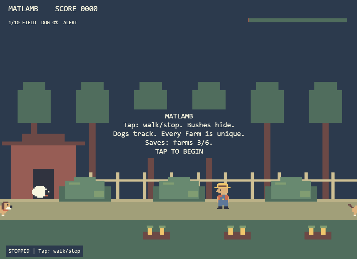
(If you would like a tutorial on the game, make sure to check out my other Tips & Tricks post!)
The Idea
When I started brainstorming ideas, I knew I wanted to do something fun Mathworks related. After spending a few days brainstorming ideas and getting nowhere, I finally found my inspiration in this perfectly timed Mathworks Instagram Post! There is an actual sheep born in 2024 at Mass Audubon's Drumlin Farm in Massachusetts and named in honor of MathWorks. Apparently, some of the sheep escaped their barn, and MATLAMB was suspected of leading the charge! You literally cannot make up a better MATLAB game idea.
Designing around one button
My biggest design challenge was making a stealth game that still requires strategy without having separate movement and hiding controls.
I decided to make the sheep move automatically when walking is toggled on. Instead of controlling its direction, players have to observe the farmers movements and make tactical decisions on when to stop.
However, I quickly realized that players could just camp in bushes until the perfect opportunity to move, which took away much of the challenge. So, how did I fix this? Puppies! No, literally. I added dogs that follow the sheep's trail and sniff out its hiding spots, forcing players to keep moving instead of staying in one bush forever.
To prevent the game from feeling repetitive, I gave the ten sections, aka 'farms' different mechanics. These include a farmer with a lantern that detects movement in both directions, muddy terrain that reduces movement speed, and a windmill farm where changing wind directions can push the sheep even when the player stops.
Working with AI and the character limit
I used ChatGPT throughout development to help write, revise, and simplify the MATLAB code. I guided the game's design and continued adjusting the mechanics, enemy behavior, difficulty, and overall gameplay.
One of the hardest constraints was the 10,000-character limit. As I added more mechanics, I had to find ways to reduce the code size without removing the features that made the game interesting.
Some useful approaches included shortening internal variable names, representing multiple enemies with arrays, using shared functions for repeated graphics operations, and constructing scenery from reusable patterns.
My biggest takeaway was that the one-button restriction actually encouraged me to design more creative game mechanics.
I'd be interested to hear how other participants approached one-button game design in MATLAB!
Thank you for taking the time to read my post, best of luck to you all!

This Week's Quiz
403 responses

For the MATLAB One-Button Game Mini Hack, I created RESONANCE — Master the Frequency, a five-level educational game that transforms a simple physics simulation into an interactive challenge.
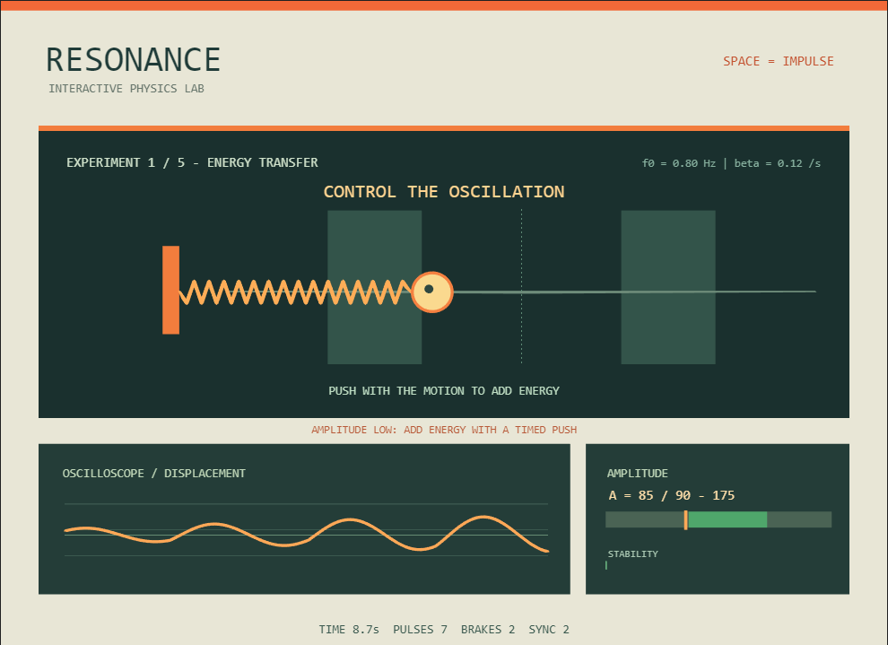
RESONANCE — An interactive mass–spring–damper experiment controlled with a single button.
The idea started with a question:
Can someone learn how oscillations work by controlling them with only one button?
Instead of directly moving a character, the player applies impulses to a mass–spring–damper system. Depending on the timing, an impulse can increase or decrease the oscillator's mechanical energy.
The challenge is not to press the button as fast as possible. It is to understand when to press it and why the timing matters.
1. Turning a Physics Equation into Gameplay
RESONANCE is based on the classical mass–spring–damper system.
Its equation of motion is:
m*x'' + c*x' + k*x = F(t)
where:
- m represents mass.
- c is the damping coefficient.
- k represents spring stiffness.
- x is displacement.
- F(t) is the externally applied force.
Between impulses, the game uses the normalized equation for unit mass:
x'' + 2*beta*x' + omega_0^2*x = 0
Here, beta controls damping and omega_0 represents the undamped natural angular frequency.
The simulation uses a compact numerical integration method:
s.v=s.v+(-s.w^2*s.x-2*s.beta*s.v)*dt;
s.x=s.x+s.v*dt;
These two lines update velocity and displacement using a semi-implicit Euler method.
One useful discovery was that changing just a few physical parameters could create very different gameplay challenges.
Increasing damping makes the oscillator lose energy faster. Increasing natural frequency makes the motion faster, forcing the player to adjust the timing of their impulses.
This allowed me to build several levels around the same physical model.
2. One Button, Two Different Energy Outcomes
The main mechanic is surprisingly simple: pressing SPACE applies an impulse toward the right.
The corresponding MATLAB code is:
s.delta=s.v*s.j+.5*s.j^2;
s.v=s.v+s.j;
The change in mechanical energy caused by an instantaneous velocity impulse, assuming unit mass, is:
Delta_E = v*J + 0.5*J^2
Here, v is the velocity before the impulse and J is the velocity increment.
This produces an interesting result:
- When the mass moves to the right, a rightward impulse increases its kinetic energy.
- When the mass moves sufficiently fast to the left, the same impulse reduces its kinetic energy.
- If the mass moves too slowly to the left, the impulse can reverse its direction and still increase its energy.
In other words, the same button can accelerate or brake the oscillator depending on its current motion.
The player gradually discovers this relationship through experimentation.
This became the foundation of the game's educational design.
3. Measuring Amplitude Through Energy
Another important challenge was determining whether the player had successfully controlled the oscillator.
Instead of checking only the mass's position, the game calculates an energy-based amplitude indicator:
s.A=sqrt(s.x^2+(s.v/s.w)^2);
For the corresponding undamped oscillator with unit mass, mechanical energy is:
E = 0.5*v^2 + 0.5*omega_0^2*x^2
From this expression, an equivalent amplitude can be calculated:
A = sqrt(x^2 + (v/omega_0)^2)
In the damped simulation, this serves as an instantaneous energy-based amplitude indicator rather than an exact prediction of the next displacement peak.
The player must maintain this indicator within a specified target range for a certain amount of time.
This creates an interesting challenge: reaching the correct amplitude is only part of the solution. The player must also prevent the system from gaining or losing too much energy.
4. Designing Five Educational Levels
I organized RESONANCE into five experiments, each introducing a different learning objective.
Level 1 — Energy Transfer
The player learns how properly timed impulses can increase the oscillator's energy and amplitude.
This first level introduces the basic relationship between motion, timing, and energy transfer.
Level 2 — Damping
The damping coefficient increases, causing the oscillator to lose energy more rapidly.
The player must compensate for that loss by applying impulses at appropriate moments.
The objective is to understand that maintaining an oscillation requires replacing the energy dissipated by damping.
Level 3 — Precision Control
The player must apply at least one impulse that reduces mechanical energy.
This level introduces active braking and demonstrates that applying more force is not always the correct solution.
Sometimes the best action is to remove energy.
Level 4 — Natural Frequency
The oscillator's natural frequency increases.
Its oscillations become faster, giving the player less time to react.
The challenge includes two phase-aligned impulses, encouraging the player to adapt to the system's changing dynamics.
Level 5 — Resonance Challenge
The final experiment requires three phase-aligned impulses followed by precise amplitude stabilization.
The game recognizes favorable impulses near the equilibrium position while the mass is moving toward the right:
if s.v>0 && abs(s.x)<40
s.sync=s.sync+1;
end
This demonstrates how the timing of repeated energy transfers influences the buildup of oscillations.
Classical resonance involves periodic excitation near a system's natural frequency. RESONANCE uses discrete impulses instead, providing a simplified, interactive analogy of phase-synchronized excitation rather than a complete simulation of sinusoidal resonance.
5. Making Physics Visible
I wanted RESONANCE to look like an interactive physics laboratory rather than a traditional arcade game.
The interface includes:
- An animated mass connected to a spring.
- An oscilloscope-style displacement trace.
- Highlighted target amplitude regions.
- A real-time amplitude indicator.
- A stability progress bar.
- Feedback about energy transfer and impulse timing.
One useful MATLAB technique was creating the graphics objects during initialization and updating their properties during gameplay.
For example, the spring animation uses:
s.coil.XData=linspace(161,p-20,32);
s.coil.YData=271+[0 repmat([10 -10],1,15) 0];
This changes the spring's geometry as the mass moves, creating the appearance of stretching and compression.
The oscilloscope provides another view of the same physical process, helping the player connect the moving mass with its displacement over time.
These visual elements are not merely decorative. They help communicate the behavior of the underlying system.
6. Learning Through Feedback
An important lesson during development was that a game does not automatically become educational just because it contains a physics simulation.
The player needs enough information to understand what is happening.
I therefore introduced contextual feedback during gameplay.
For example, when the amplitude is too low, the game suggests adding energy with a well-timed impulse. When the amplitude is too high, it encourages the player to consider braking.
The game also displays a short explanation after each completed experiment.
The player must press SPACE to continue, allowing time to read the explanation before starting the next challenge.
This creates a simple learning cycle:
Experiment → Observe → Adjust → Succeed → Understand
Rather than presenting equations as a separate lesson, the game connects the explanations to actions the player has already performed.
7. Working Within the 10,000-Character Limit
One of the biggest technical challenges was fitting the physics simulation, five levels, graphics, gameplay logic, and educational messages within the contest's 10,000-character limit.
To keep the implementation compact, I:
- Reused the same graphics objects across all levels.
- Stored level-specific parameters in arrays.
- Used small helper functions for drawing.
- Kept the physics calculations separate from rendering.
- Avoided unnecessary dependencies and additional game files.
The published version contains 9,305 characters according to the official MATLAB contest validator.
A useful lesson from this process was to rely on minihackContest.validate instead of estimating the character count from the source file, because the validator applies its own counting rules.
The character limit also encouraged me to focus on the mechanics that contributed most to gameplay and learning.
8. Development Process and Lessons Learned
AI assistance was used during concept development, MATLAB code generation, debugging, and iterative refinement.
I tested the game in MATLAB, evaluated the difficulty of each experiment, adjusted parameters, refined the educational messages, and validated the implementation using the official contest tools.
One challenge was balancing the difficulty progression.
During early testing, the damping experiment and the final synchronization challenge were particularly demanding. Adjusting the target ranges and stability requirements helped create a more gradual progression.
Another important decision was to distinguish between the physics being simulated directly and the concepts being demonstrated through simplified gameplay.
The main lessons I took from this project were:
- A differential equation can become the foundation of an engaging game mechanic.
- A single input can produce different physical outcomes depending on the system's state.
- Visualizing displacement and amplitude can make abstract concepts easier to understand.
- Increasing difficulty works best when each level builds on previously learned skills.
- Educational feedback is most meaningful when it explains something the player has just experienced.
Final Thoughts
RESONANCE is an experiment in combining simulation, game design, and STEM education within a very small MATLAB project.
The goal was not to create the most complicated physics simulator, but to make a few important concepts intuitive through interaction.
By the end of the five experiments, I hope players have developed a better intuition for energy transfer, damping, natural frequency, and the importance of impulse timing.
Sometimes, the best way to understand a physical system is to try controlling it.
Thanks for reading, and I hope you enjoy experimenting with RESONANCE!
A huge thank you to everyone who participated in the MATLAB STEM Showcase!
What makes these contributions especially meaningful is that their impact doesn’t end with the contest. Your work can continue to help students, educators, engineers, scientists, and curious learners explore STEM concepts for years to come.
And now, it’s time to celebrate our winners!
🥇 STEM Domain Awards
Congratulations to our STEM Domain Award winners. Each of you will receive a $50 Amazon gift card.
AI & Data Science:
@Yiheng for Inside the VAE
Physics:
Mathematics:
Engineering:
Life Sciences:
Earth & Climate Science:
🎁 Weekly Prize Winners
Congratulations as well to all of our Weekly Prize winners! You will receive a MathWorks T-shirt or a pair of socks.
@Anshika, @Jan Studnicka, @Michelle, @Abhishek, @Dr. Mishaal A. AbdulKareem, @Harshad, @KARUPPASAMYPANDIYAN M, @Umar, @Heze Chen, @Jamil Kasan, @Jorge Paloschi, @Pauli Huusari, @Rodolfo
Congratulations to all our winners, and thank you again to everyone who participated!
We hope you’ll continue creating, exploring, and sharing interactive STEM experiences with the MATLAB community.

What does the participation matrix represent - from the Modern Grid Stability with IBRs: Leveraging Simulation and Control Design session.
FOLD: One Button, Two Worlds
For the MATLAB One-Button Game Mini Hack, I developed FOLD, a six-level puzzle-platformer built entirely in MATLAB.
Unlike traditional platformers, the player does not directly control the character. Instead, the character moves automatically, while a single button changes the geometry of the environment.
Each press rotates platforms, changes available paths, and activates or deactivates obstacles.
Play FOLD here:
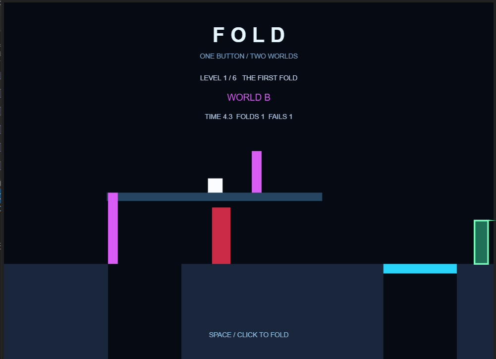
FOLD — Rotating platforms and phase-based obstacles controlled with a single button.
1. Creating Rotating Platforms with Trigonometry
One of the main technical challenges was creating platforms that rotate around a fixed pivot.
Rather than recreating graphical objects every frame, I calculate the vertices of each platform using trigonometric functions.
For a platform with length L, thickness w, and rotation angle a:
dx=L*cos(a);
dy=-L*sin(a);
nx=w*sin(a);
ny=w*cos(a);
px=[x x+dx x+dx+nx x+nx];
py=[y y+dy y+dy+ny y+ny];
These coordinates define the four corners of the platform.
By updating the XData and YData properties of an existing patch, MATLAB can animate the platform without creating new graphics objects every frame.
This approach keeps the animation simple and efficient.
2. Making the Character Move with a Platform
Initially, the character would fall whenever a platform started rotating.
To solve this, I introduced a mechanism that temporarily attaches the character to the rotating platform.
The character's position is calculated relative to the platform's pivot:
s.x=170+s.dist*cos(a)-12;
s.y=440-s.dist*sin(a)-24;
Here, s.dist represents the distance along the platform, while a is the current rotation angle.
This allows the character to move together with the platform and reach elevated sections of the level.
3. Designing Gameplay Around a Single Button
The most interesting design challenge was creating meaningful gameplay with only one input.
FOLD uses two world states: A and B.
Pressing SPACE or clicking the mouse switches between these states. Multiple platforms respond simultaneously, while certain obstacles become active or inactive.
This creates situations where opening one path may close another.
Across six levels, players must learn to anticipate how their actions affect the environment.
The objective was to make the game progressively more strategic without introducing additional controls.
4. Optimizing MATLAB Code for the Character Limit
The competition limits submissions to 10,000 characters.
One important discovery was that the validator's character count could differ significantly from the raw source file length.
Removing whitespace alone was not sufficient.
I reduced code duplication, reused helper functions, represented level configurations using arrays, and simplified unnecessary graphical elements.
The final implementation successfully passed minihackContest.validate.
5. What I Learned
Developing FOLD helped me explore several useful MATLAB techniques:
- Updating existing graphical objects instead of recreating them.
- Applying trigonometry to interactive 2D geometry.
- Managing game states and frame-based updates.
- Designing multiple puzzles around a single input.
- Optimizing code under strict technical constraints.
AI assistance was used during prototyping, debugging, and code refinement. The gameplay was tested locally in MATLAB, and the final submission passed the official contest validator.
The main takeaway: limitations can encourage creativity. With a single button, basic trigonometry, and carefully designed state transitions, it is possible to build an interactive puzzle game with surprisingly varied gameplay.
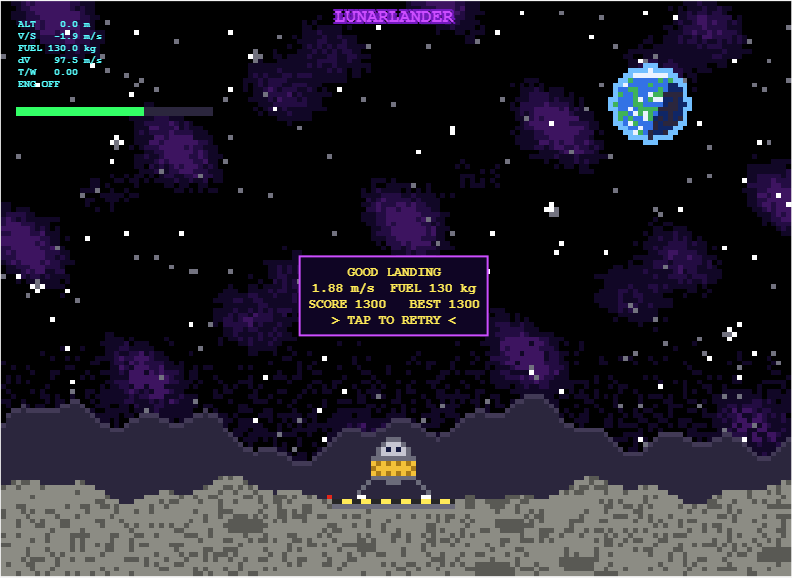
My entry for the one-button game mini hack Lunar Lander - Tap to Burn, is a one-button powered descent. You start 500 m above the surface, falling at 10 m/s, with 200 kg of propellant. One tap turns on the engine, and the next tap stops it.
How scoring works
- Crash: landing at 3 m/s or faster scores 0.
- Abort: rising above 750 m scores 0.
- Safe landing: below 3 m/s scores 10 points per kilogram of fuel remaining.
- Perfect touchdown: below 1 m/s doubles the reward to 20 points per kilogram of fuel remaining.
Physics in the game
- Fuel mass decreases as propellant is burned.
- Gravity continuously accelerates the lander downward.
- The engine does not reach full thrust instantly, so timing matters.
- The display turning red indicates when a full thrust landing burn becomes possible.
Display readouts
- ALT [m]: Height above the surface.
- V/S [m/s]: Vertical speed.
- FUEL [kg]: Remaining propellant.
- dV [m/s]: remaining velocity change the fuel can provide, from the rocket equation Δv=Isp·g₀·ln(m/m_dry).
- T/W: Thrust to weight ratio.
My best so far is 1300. Has anyone managed a sub 1m/s landing?

I thought I had the game in pretty good shape until I tried it in MATLAB Online. A launch that felt immediate on desktop could feel slower in the browser, which matters in a game where timing is the main control.
I built Slingshot Home: Escape Saturn for the MATLAB One-Button Game Mini Hack. The goal is to time your launches to travel between 15 of Saturn’s moons and return to Earth, with three shields and a clock counting down.
Getting the game to feel responsive took a few iterations, particularly when running it in MATLAB Online. Here are some of the approaches that worked well.
Reuse Graphics Objects
The game creates 21 graphics objects during initialization and reuses them throughout gameplay. Instead of recreating the scene, it updates properties such as position, color, and text.
I also check whether a property has changed before assigning it again. Static planets and labels do not need to be updated as frequently as the spacecraft.
For the Mini Hack, the game harness handles the window, input, and drawing loop. The game provides the init, update, and render functions.
Use Elapsed Time for Motion
The spacecraft moves around each moon using basic trigonometry:
theta = startAngle + angularSpeed*elapsedTime;
position = moonCenter + radius*[cos(theta), sin(theta)];
heading = [-sin(theta), cos(theta)];
Pressing the button launches the spacecraft along the tangent to its current orbit, so the gameplay is based on timing rather than steering.
Calculating the orbital angle from elapsed game time, rather than advancing it by a fixed amount per frame, also makes the motion less dependent on rendering speed.
Separate Trajectory Calculation from Rendering
I used ode45 to calculate each flight trajectory, then deval and interpolation to provide positions during playback. This avoids solving the trajectory again on every frame.
The physics is intentionally simplified. The moons remain in fixed positions, captures are assisted, and the escape gate represents leaving Saturn’s sphere of influence rather than calculating its actual boundary. These assumptions are documented in the code comments.
Generate Textures in MATLAB
The planet textures are generated directly in MATLAB, so there are no external image files to load:
MATLAB
x = linspace(-1,1,80);
z = max(0,1-x.^2-x'.^2);
brightness = max(.1,.8*sqrt(z)-.6*x);
This produces directional lighting while retaining some brightness on the night side. The textures are generated once during initialization.
Increasing the texture resolution helped smooth the edges, but adjusting the lighting had a larger effect on the overall appearance.
Test as You Go
I used Codex to help edit and refine the code. Through MATLAB MCP, it could run MATLAB code, inspect Code Analyzer results, and exercise states such as countdown, launch, and restart.
That was useful for finding issues, but running and playing the game was still important. Some things only became apparent during gameplay, such as a launch feeling delayed or an orbit being difficult to see. I also tested regularly in MATLAB Online rather than relying only on desktop behavior.
I used the Mini Hack validator to keep track of the character limit:
minihackContest.validate
The validator count differs from the raw file size. Comments are excluded, so I could document the physics and assumptions without using the executable-code budget.
Try It in MATLAB Online
One feature I liked about the final result is that there is very little setup required to try it.
Click “Play game,” then “Run this app,” and the game runs in the browser.
For me, the biggest improvements came from fairly small changes: reusing graphics objects, basing motion on elapsed time, calculating trajectories separately from rendering, and testing regularly in MATLAB Online.

My second entry, Event Horizon (entry 16546), puts you in orbit around a black hole. Tapping fires your engine and climbs, and the accretion disk's drag pulls you down. Lower orbits slow your clock, so your score is how many years into Earth's future you travel. Flares light up rings of the disk, and you have to get out of a red band before it turns white and burns.
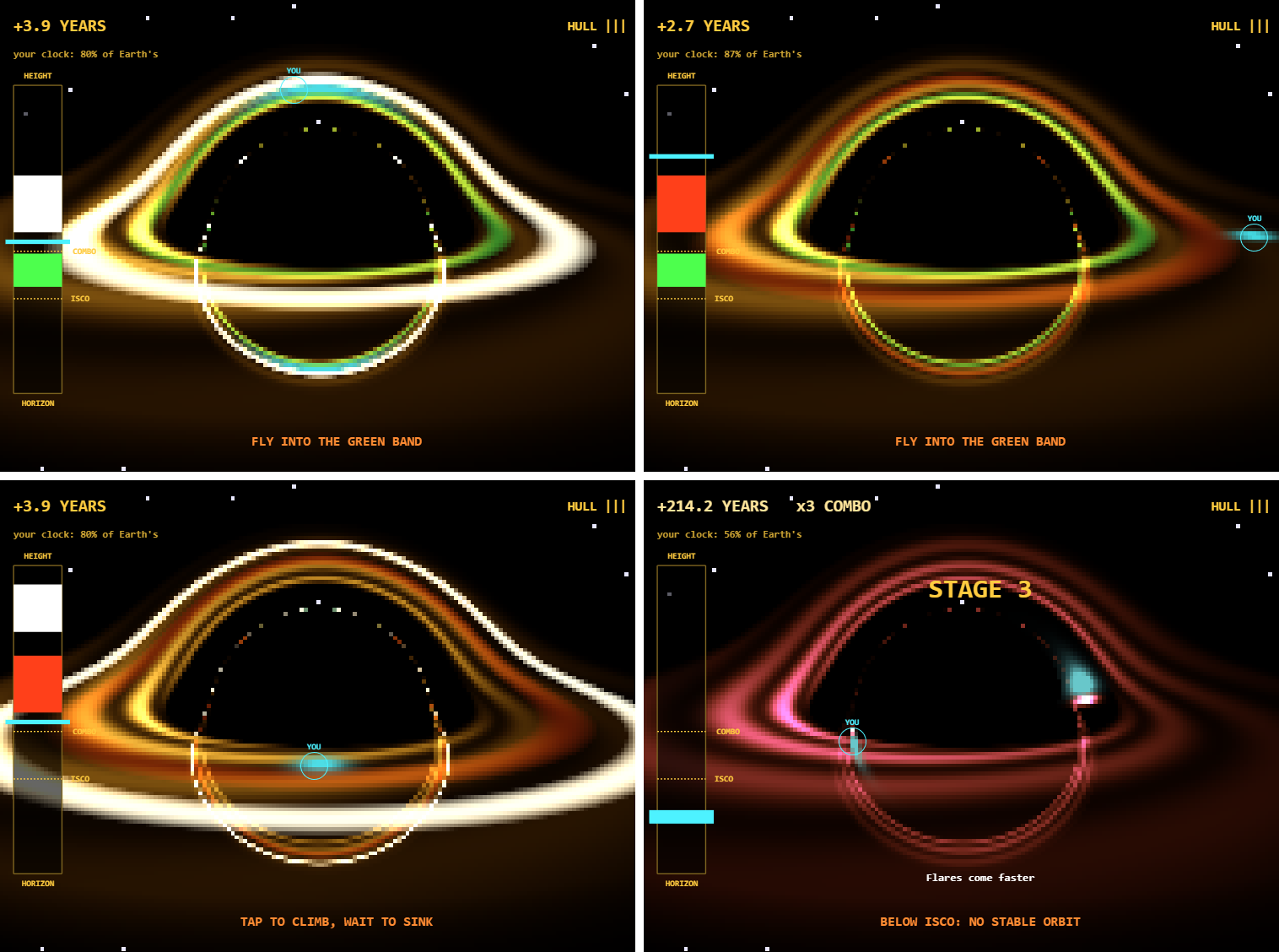
Real frames from the game. In the top left, the ship (cyan, marked YOU) is behind the hole, and gravity bends its light into an arc over the top.
The picture isn't drawn by hand. It comes from tracing light through the Schwarzschild metric, the spacetime around a non-spinning black hole. Here is what I learned building it, again with help from an AI coding assistant (Claude Code), testing each change in MATLAB.
1. Trace the light once, then shade the map every frame
My first prototype traced one light ray per pixel every frame. With rays bending around the hole, that took about 240 ms per frame at 160 by 120 pixels, far over the 33 ms a 30 fps frame allows.
The fix was to notice that the camera never moves. Each pixel's ray always lands in the same place, so I trace every ray once in init and store where it crosses the plane of the disk. In these units, with the Schwarzschild radius set to 1, a light ray's path follows a simple force law, which I step for all 19,200 rays at once:
h2 = sum(cross(P,V).^2); % each ray's angular momentum squared
for k = 1:150
d = min(.07*vecnorm(P),1); % smaller steps near the hole
Q = P+V.*d;
V = V-1.5*h2.*Q./vecnorm(Q).^5.*d;
% ...record where each ray crosses z = 0, drop rays that escape or fall in
end
Each ray keeps its first two crossings of the disk plane. The first is the direct view. The second is light that went around the back of the hole, which is why you can see the far side of the disk both above and below the shadow.
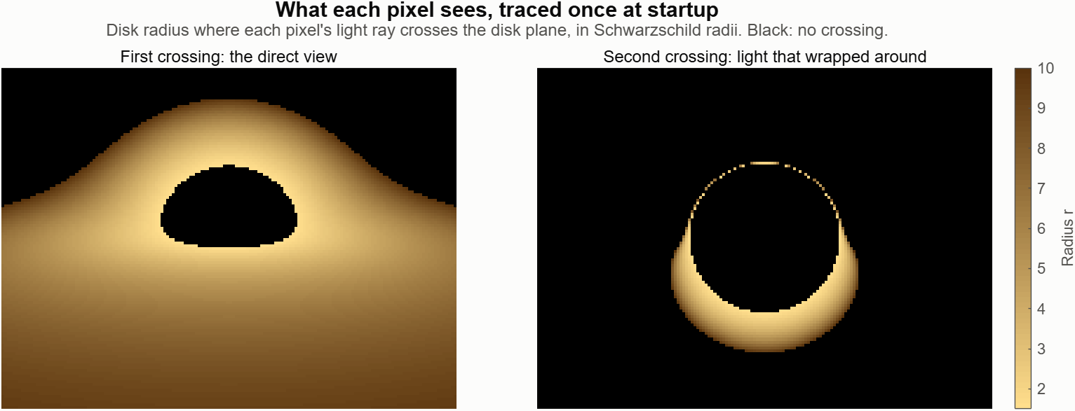
The trace takes about 160 ms at startup on my PC. After that, each frame only shades the stored points, and the game's whole frame work is about 6 ms.
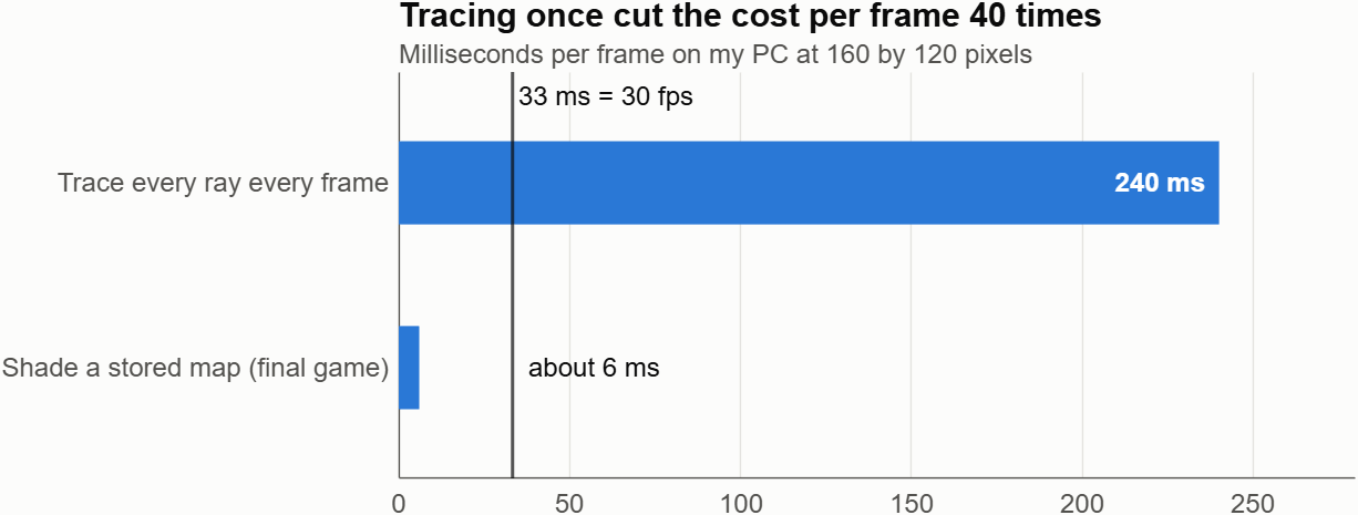
The 240 ms comes from an early prototype with a slightly different camera, so treat the ratio as approximate.2. Paint the game into the disk, and gravity bends it for free
Because the map stores a disk position for every pixel, anything I draw in disk coordinates gets lensed automatically. The ship is just a glow centered on its position in the disk, and the flares are rings of disk radius:
zs = s.r*exp(1i*s.ph); % ship position as x + iy
S(L.i) = S(L.i)+exp(-abs(L.c-zs).^2/.2); % L.c: disk point of each pixel
b = max(0,1-((L.r-s.fc)./s.fw).^2); % flare rings by radius
When the ship passes behind the hole, its image smears into arcs above and below the shadow. No extra code does that. The engine exhaust from each tap is drawn the same way, so it bends too.
Storing disk points as complex numbers kept the distance check to one short line.
3. Real physics needed a real gauge
The orbit uses the Schwarzschild radial equation, so the innermost stable orbit at r = 3 is real: below it, no orbit is stable and the ship slides inward. Time dilation sets the score. A circular orbit's clock runs at sqrt(1 - 1.5/r) of a distant clock, so Earth gains the rest:
s.vr = s.vr+(-.5/s.r^2+s.L^2/s.r^3-1.5*s.L^2/s.r^4-.04*s.vr)*T;
s.yrs = s.yrs+10*h*s.m*(1-sqrt(max(0,1-1.5/s.r)));
The physics made two first designs fail:
- Head-on debris didn't work. Moving up or down is slower than going around the hole, so you met debris before a burn could lift you clear. Climbing one unit took about 3 s even tapping 5 times a second. I replaced debris with flares that warn for 3.5 s, and I sped up game time 1.6 times.
- A beautiful view isn't a readable one. In my first playtest, I couldn't tell what a tap did, because the lensed ship jumps around the screen. A simple height gauge on the left fixed that. Tapping moves your bar up, red bands are flares, and green bands are bonuses. The black hole is the show, and the gauge is the controller.
After that came the parts that made it fun: a combo multiplier for staying deep, stages every 100 years with faster and drifting flares, and a close-call bonus for clearing a flare by a hair.4. Small tricks that saved characters
The final file counts 9,993 of 10,000 characters. The counter reformats your code first, so comments are free but spaces and indentation count, as I described in my first post. These helped:
- Divide by zero to hide things. 0/0 is NaN, and graphics skip NaN points, so one expression both positions and hides a marker:G.gs.YData = [1 1]*(100+60*(s.r-1))+0/(s.mode == 1);
- Make several texts in one call. text takes vectors and a cell array of strings:text(ax,[103 108 50 50],[220 280 88 502],{'ISCO','COMBO','HORIZON','HEIGHT'},f{:});
- Store end times, not countdowns. A message that shows until s.t < s.got needs no line to count it down each frame.
- Write constants out when they're fixed. My camera never moves, so its right and up vectors became constants instead of cross products.
One trim I had to undo: dropping a normalization in the star placement put stars inside the black hole's shadow. Look at the frames after every trim.Play it
If MATLAB Online is slow for you, run it in desktop MATLAB: download the starter project, copy the entry's code into game.m, and run minihackContest.play.
How many years into the future can you get?

Lira vanished 19 years ago. Now her signal is back. You control a radio telescope that sweeps the sky, and you only have one button (SPACE or click).
- Watch the dish sweep left and right. When the beam passes over a “?” in the sky, press to lock onto the signal.
- Then tap as fast as you can to collect pulses (up to 8 in 2.4 seconds).
- Each signal turns out to be an ALIEN, a NEW PLANET or a BLACK HOLE, and a little face appears in the sky.
- Lira’s signature is SHORT-SHORT-LONG. Aliens repeat it, so they need more pulses to be confirmed. If you don’t reach the goal, the alien gets away and you can try again.
- Every alien you confirm decodes part of a hidden message. Clear the three sectors (Pulsar, Dust Cloud, Deep Space) to read it.
HOW THE CODE WORKS
The game follows the contest contract: game() returns init, update and render.
1. init – builds everything once.
It draws the pixel-art backdrop (one small image with a sunset in color bands), the dish, the wave panel, the texts and the three faces. Each face is a few ellipse patches inside an hggroup, parented to an hgtransform so it can be moved and scaled later.
2. update – the game logic.
The game is a small state machine with one phase number: 0 ready, 1 scan, 2 collect, 3 transit, 4 done. The same button means “start”, “lock on” or “tap fast” depending on the phase. A short cooldown after each press avoids double hits.
The dish angle is a triangle wave over time:
a = 110*(1-abs(mod(t*rate/110,2)-1))-55
A target can be locked when it is within 14 degrees of the beam. Each sector raises the sweep rate.
3. Signals and their type.
Each signal is built from two 3-letter patterns of short (S) and long (L) pulses, drawn as one waveform. The type comes straight from the patterns:
- both halves equal to Lira’s SSL → alien
- both halves equal but different → new planet
- halves different → black hole
So the wave you see on screen really tells you what you found.
4. render – only updates properties.
Nothing is created while playing. Each frame only changes XData/YData of the dish and wave, the String and Color of the texts, and the Matrix of each face (makehgtform with translate and scale). The faces “pop” on every tap with a simple scale change. This keeps the game smooth.
5. Fitting under 10,000 characters.
The validator counted more than the file size, so I used anonymous helpers for repeated line/text calls, stored shapes in small matrices and ran minihackContest.validate often.
Thanks for playing, and good luck everyone!

Thanks to Dr. Riyadh Kenaya and Arnie Berlin for the session and for answering my questions live: UE5 handles radial and tangential distortion, rolling shutter would be added in Simulink, and the synthetic data is meant for design of experiments on extrinsic limits rather than exact calibration.
A few follow-ups:
- The demo results showed a mean calibration error of 3.85 px, with camera 1 at 7.33 px. On synthetic images where the true intrinsics are known, what drives that error: the distortion model fit, board detection near the image edges, or something else?
- Can the ChArUco board poses be set from a script instead of the Control Center sliders? That would let a calibration campaign run as a Monte Carlo sweep over board placement and lighting.
- Does the camera model support fisheye or rational distortion models for wide lenses (around 100 degrees horizontal)?
- With a 32-channel lidar, only a few rings hit each board. How much does camera-to-lidar extrinsic accuracy degrade as the boards move farther away?
I would also be glad to try the example if the code is available.
Discussions 정보
Discussions is a user-focused forum for the conversations that happen outside of any particular product or project.
Get to know your peers while sharing all the tricks you've learned, ideas you've had, or even your latest vacation photos. Discussions is where MATLAB users connect!
Get to know your peers while sharing all the tricks you've learned, ideas you've had, or even your latest vacation photos. Discussions is where MATLAB users connect!
기타 커뮤니티 영역

MATLAB Answers
MATLAB 및 Simulink에 관해 묻고 답하세요!

File Exchange
사용자 제출 코드를 다운로드하고 기여하세요!

Cody
문제를 풀고 MATLAB에 대해 배우며 배지도 획득하세요!

블로그
내부 개발자가 바라보는 MATLAB 및 Simulink!

AI Chat Playground
AI를 사용해 MATLAB 코드 초안을 생성하고 질문에 답할 수 있습니다!

