Main Content

compareHoldout

Compare accuracies of two classification models using new data

Description

compareHoldout statistically assesses the accuracies of two classification models. The function first compares their predicted labels against the true labels, and then it detects whether the difference between the misclassification rates is statistically significant.

You can determine whether the accuracies of the classification models differ or whether one model performs better than another. compareHoldout can conduct several McNemar test variations, including the asymptotic test, the exact-conditional test, and the mid-p-value test. For cost-sensitive assessment, available tests include a chi-square test (requires Optimization Toolbox™) and a likelihood ratio test.

example

h = compareHoldout(C1,C2,T1,T2,ResponseVarName) returns the test decision from testing the null hypothesis that the trained classification models C1 and C2 have equal accuracy for predicting the true class labels in the ResponseVarName variable. The alternative hypothesis is that the labels have unequal accuracy.

The first classification model C1 uses the predictor data in T1, and the second classification model C2 uses the predictor data in T2. The tables T1 and T2 must contain the same response variable but can contain different sets of predictors. By default, the software conducts the mid-p-value McNemar test to compare the accuracies.

h = 1 indicates rejecting the null hypothesis at the 5% significance level. h = 0 indicates not rejecting the null hypothesis at the 5% level.

The following are examples of tests you can conduct:

  • Compare the accuracies of a simple classification model and a model that is more complex by passing the same set of predictor data (that is, T1 = T2).

  • Compare the accuracies of two potentially different models using two potentially different sets of predictors.

  • Perform various types of Feature Selection. For example, you can compare the accuracy of a model trained using a set of predictors to the accuracy of one trained on a subset or different set of those predictors. You can choose the set of predictors arbitrarily, or use a feature selection technique such as PCA or sequential feature selection (see pca and sequentialfs).

h = compareHoldout(C1,C2,T1,T2,Y) returns the test decision from testing the null hypothesis that the trained classification models C1 and C2 have equal accuracy for predicting the true class labels Y. The alternative hypothesis is that the labels have unequal accuracy.

The first classification model C1 uses the predictor data T1, and the second classification model C2 uses the predictor data T2. By default, the software conducts the mid-p-value McNemar test to compare the accuracies.

example

h = compareHoldout(C1,C2,X1,X2,Y) returns the test decision from testing the null hypothesis that the trained classification models C1 and C2 have equal accuracy for predicting the true class labels Y. The alternative hypothesis is that the labels have unequal accuracy.

The first classification model C1 uses the predictor data X1, and the second classification model C2 uses the predictor data X2. By default, the software conducts the mid-p-value McNemar test to compare the accuracies.

example

h = compareHoldout(___,Name,Value) specifies options using one or more name-value pair arguments in addition to the input argument combinations in previous syntaxes. For example, you can specify the type of alternative hypothesis, specify the type of test, and supply a cost matrix.

example

[h,p,e1,e2] = compareHoldout(___) returns the p-value for the hypothesis test (p) and the respective classification losses of each set of predicted class labels (e1 and e2) using any of the input arguments in the previous syntaxes.

Examples

collapse all

Train two k-nearest neighbor classifiers, one using a subset of the predictors used for the other. Conduct a statistical test comparing the accuracies of the two models on a test set.

Load the carsmall data set.

load carsmall

Create two tables of input data, where the second table excludes the predictor Acceleration. Specify Model_Year as the response variable.

T1 = table(Acceleration,Displacement,Horsepower,MPG,Model_Year);
T2 = T1(:,2:end);

Create a partition that splits the data into training and test sets. Keep 30% of the data for testing.

rng(1)  % For reproducibility
CVP = cvpartition(Model_Year,'holdout',0.3);
idxTrain = training(CVP);   % Training-set indices
idxTest = test(CVP);    % Test-set indices

CVP is a cross-validation partition object that specifies the training and test sets.

Train the ClassificationKNN models using the T1 and T2 data.

C1 = fitcknn(T1(idxTrain,:),'Model_Year');
C2 = fitcknn(T2(idxTrain,:),'Model_Year');

C1 and C2 are trained ClassificationKNN models.

Test whether the two models have equal predictive accuracies on the test set.

h = compareHoldout(C1,C2,T1(idxTest,:),T2(idxTest,:),'Model_Year')
h = logical
   0

h = 0 indicates to not reject the null hypothesis that the two models have equal predictive accuracies.

Train two classification models using different algorithms. Conduct a statistical test comparing the misclassification rates of the two models on a test set.

Load the ionosphere data set.

load ionosphere

Create a partition that evenly splits the data into training and test sets.

rng(1)                             % For reproducibility
CVP = cvpartition(Y,'holdout',0.5);
idxTrain = training(CVP);           % Training-set indices 
idxTest = test(CVP);                % Test-set indices

CVP is a cross-validation partition object that specifies the training and test sets.

Train an SVM model and an ensemble of 100 bagged classification trees. For the SVM model, specify to use the radial basis function kernel and a heuristic procedure to determine the kernel scale.

C1 = fitcsvm(X(idxTrain,:),Y(idxTrain),'Standardize',true, ...
    'KernelFunction','RBF','KernelScale','auto');
t = templateTree('Reproducible',true);  % For reproducibility of random predictor selections
C2 = fitcensemble(X(idxTrain,:),Y(idxTrain),'Method','Bag', ...
    'Learners',t);

C1 is a trained ClassificationSVM model. C2 is a trained ClassificationBaggedEnsemble model.

Test whether the two models have equal predictive accuracies. Use the same test-set predictor data for each model.

h = compareHoldout(C1,C2,X(idxTest,:),X(idxTest,:),Y(idxTest))
h = logical
   0

h = 0 indicates to not reject the null hypothesis that the two models have equal predictive accuracies.

Train two classification models using the same algorithm, but adjust a hyperparameter to make the algorithm more complex. Conduct a statistical test to assess whether the simpler model has better accuracy on test data than the more complex model.

Load the ionosphere data set.

load ionosphere;

Create a partition that evenly splits the data into training and test sets.

rng(1);                             % For reproducibility
CVP = cvpartition(Y,'holdout',0.5);
idxTrain = training(CVP);           % Training-set indices 
idxTest = test(CVP);                % Test-set indices

CVP is a cross-validation partition object that specifies the training and test sets.

Train two SVM models: one that uses a linear kernel (the default for binary classification) and one that uses the radial basis function kernel. Use the default kernel scale of 1.

C1 = fitcsvm(X(idxTrain,:),Y(idxTrain),'Standardize',true);
C2 = fitcsvm(X(idxTrain,:),Y(idxTrain),'Standardize',true,...
    'KernelFunction','RBF');

C1 and C2 are trained ClassificationSVM models.

Test the null hypothesis that the simpler model (C1) is at most as accurate as the more complex model (C2). Because the test-set size is large, conduct the asymptotic McNemar test, and compare the results with the mid-p-value test (the cost-insensitive testing default). Request to return p-values and misclassification rates.

Asymp = zeros(4,1); % Preallocation
MidP = zeros(4,1); 

[Asymp(1),Asymp(2),Asymp(3),Asymp(4)] = compareHoldout(C1,C2,...
    X(idxTest,:),X(idxTest,:),Y(idxTest),'Alternative','greater',...
    'Test','asymptotic');
[MidP(1),MidP(2),MidP(3),MidP(4)] = compareHoldout(C1,C2,...
    X(idxTest,:),X(idxTest,:),Y(idxTest),'Alternative','greater');
table(Asymp,MidP,'RowNames',{'h' 'p' 'e1' 'e2'})
ans=4×2 table
            Asymp          MidP   
          __________    __________

    h              1             1
    p     7.2801e-09    2.7649e-10
    e1       0.13714       0.13714
    e2       0.33143       0.33143

The p-value is close to zero for both tests, providing strong evidence to reject the null hypothesis that the simpler model is less accurate than the more complex model. No matter what test you specify, compareHoldout returns the same type of misclassification measure for both models.

For data sets with imbalanced class representations, or for data sets with imbalanced false-positive and false-negative costs, you can statistically compare the predictive performance of two classification models by including a cost matrix in the analysis.

Load the arrhythmia data set. Determine the class representations in the data.

load arrhythmia;
Y = categorical(Y);
tabulate(Y);
  Value    Count   Percent
      1      245     54.20%
      2       44      9.73%
      3       15      3.32%
      4       15      3.32%
      5       13      2.88%
      6       25      5.53%
      7        3      0.66%
      8        2      0.44%
      9        9      1.99%
     10       50     11.06%
     14        4      0.88%
     15        5      1.11%
     16       22      4.87%

There are 16 classes, however some are not represented in the data set (for example, class 13). Most observations are classified as not having arrhythmia (class 1). The data set is highly discrete with imbalanced classes.

Combine all observations with arrhythmia (classes 2 through 15) into one class. Remove those observations with unknown arrhythmia status (class 16) from the data set.

idx = (Y ~= '16');
Y = Y(idx);
X = X(idx,:);
Y(Y ~= '1') = 'WithArrhythmia';
Y(Y == '1') = 'NoArrhythmia';
Y = removecats(Y);

Create a partition that evenly splits the data into training and test sets.

rng(1);                             % For reproducibility
CVP = cvpartition(Y,'holdout',0.5);
idxTrain = training(CVP);           % Training-set indices 
idxTest = test(CVP);                % Test-set indices

CVP is a cross-validation partition object that specifies the training and test sets.

Create a cost matrix such that misclassifying a patient with arrhythmia into the "no arrhythmia" class is five times worse than misclassifying a patient without arrhythmia into the arrhythmia class. Classifying correctly incurs no cost. The rows indicate the true class and the columns indicate the predicted class. When you conduct a cost-sensitive analysis, a good practice is to specify the order of the classes.

cost = [0 1;5 0];
ClassNames = {'NoArrhythmia','WithArrhythmia'};

Train two boosting ensembles of 50 classification trees, one that uses AdaBoostM1 and another that uses LogitBoost. Because the data set contains missing values, specify to use surrogate splits. Train the models using the cost matrix.

t = templateTree('Surrogate','on');
numTrees = 50;
C1 = fitcensemble(X(idxTrain,:),Y(idxTrain),'Method','AdaBoostM1', ...
    'NumLearningCycles',numTrees,'Learners',t, ...
    'Cost',cost,'ClassNames',ClassNames);
C2 = fitcensemble(X(idxTrain,:),Y(idxTrain),'Method','LogitBoost', ...
    'NumLearningCycles',numTrees,'Learners',t, ...
    'Cost',cost,'ClassNames',ClassNames);

C1 and C2 are trained ClassificationEnsemble models.

Compute the classification loss for the test data by using the loss function. Specify LossFun as 'classifcost' to compute the misclassification cost.

L1 = loss(C1,X(idxTest,:),Y(idxTest),'LossFun','classifcost')
L1 = 0.6642
L2 = loss(C2,X(idxTest,:),Y(idxTest),'LossFun','classifcost')
L2 = 0.8018

The misclassification cost for the AdaBoostM1 ensemble (C1) is less than the cost for the LogitBoost ensemble (C2).

Test whether the difference is statistically significant. Conduct the asymptotic, likelihood ratio, cost-sensitive test (the default when you pass in a cost matrix). Supply the cost matrix, and return the p-values and misclassification costs.

[h,p,e1,e2] = compareHoldout(C1,C2,X(idxTest,:),X(idxTest,:),Y(idxTest),...
    'Cost',cost,'ClassNames',ClassNames)
h = logical
   0

p = 0.1180
e1 = 0.6698
e2 = 0.8093

h = 0 indicates to not reject the null hypothesis that the two models have equal predictive accuracies.

The loss function uses observation weights normalized by the prior probabilities (stored in the Prior property of the trained model), but the compareHoldout function does not use observation weights and prior probabilities. Therefore, the misclassification cost values (L1 and L2) computed by the loss function can be different from the values (e1 and e2) computed by the compareHoldout function.

Reduce classification model complexity by selecting a subset of predictor variables (features) from a larger set. Then, statistically compare the out-of-sample accuracy between the two models.

Load the ionosphere data set.

load ionosphere;

Create a partition that evenly splits the data into training and test sets.

rng(1);  % For reproducibility
CVP = cvpartition(Y,'holdout',0.5);
idxTrain = training(CVP); % Training-set indices 
idxTest = test(CVP);      % Test-set indices

CVP is a cross-validation partition object that specifies the training and test sets.

Train an ensemble of 100 boosted classification trees using AdaBoostM1 and the entire set of predictors. Inspect the importance measure for each predictor.

t = templateTree('MaxNumSplits',1); % Weak-learner template tree object
C2 = fitcensemble(X(idxTrain,:),Y(idxTrain),'Method','AdaBoostM1',...
    'Learners',t);
predImp = predictorImportance(C2);

figure;
bar(predImp);
h = gca;
h.XTick = 1:2:h.XLim(2)
h = 
  Axes with properties:

             XLim: [-0.2000 35.2000]
             YLim: [0 0.0090]
           XScale: 'linear'
           YScale: 'linear'
    GridLineStyle: '-'
         Position: [0.1300 0.1100 0.7750 0.8150]
            Units: 'normalized'

  Use GET to show all properties

title('Predictor Importance');
xlabel('Predictor');
ylabel('Importance measure');

Figure contains an axes object. The axes object with title Predictor Importance, xlabel Predictor, ylabel Importance measure contains an object of type bar.

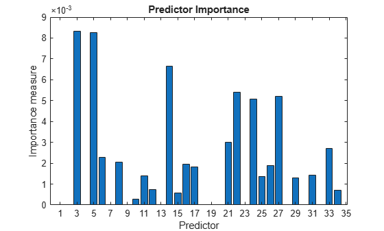
Identify the top five predictors in terms of their importance.

[~,idxSort] = sort(predImp,'descend');
idx5 = idxSort(1:5);

Train another ensemble of 100 boosted classification trees using AdaBoostM1 and the five predictors with the greatest importance.

C1 = fitcensemble(X(idxTrain,idx5),Y(idxTrain),'Method','AdaBoostM1',...
    'Learners',t);

Test whether the two models have equal predictive accuracies. Specify the reduced test-set predictor data for C1 and the full test-set predictor data for C2.

[h,p,e1,e2] = compareHoldout(C1,C2,X(idxTest,idx5),X(idxTest,:),Y(idxTest))
h = logical
   0

p = 0.7744
e1 = 0.0914
e2 = 0.0857

h = 0 indicates to not reject the null hypothesis that the two models have equal predictive accuracies. This result favors the simpler ensemble, C1.

Input Arguments

collapse all

First trained classification model, specified as any trained classification model object or compact classification model object described in this table.

Trained Model TypeModel ObjectReturned By
Classification treeClassificationTreefitctree
Discriminant analysisClassificationDiscriminantfitcdiscr
Ensemble of bagged classification modelsClassificationBaggedEnsemblefitcensemble
Ensemble of classification modelsClassificationEnsemblefitcensemble
Multiclass, error-correcting output codes (ECOC)ClassificationECOCfitcecoc
Generalized additive model (GAM)ClassificationGAMfitcgam
kNN ClassificationKNNfitcknn
Naive BayesClassificationNaiveBayesfitcnb
Neural networkClassificationNeuralNetwork (with observations in rows)fitcnet
Support vector machine (SVM)ClassificationSVMfitcsvm
Compact discriminant analysisCompactClassificationDiscriminantcompact
Compact ECOCCompactClassificationECOCcompact
Compact ensemble of classification modelsCompactClassificationEnsemblecompact
Compact GAMCompactClassificationGAMcompact
Compact naive BayesCompactClassificationNaiveBayescompact
Compact neural networkCompactClassificationNeuralNetworkcompact
Compact SVMCompactClassificationSVMcompact
Compact classification treeCompactClassificationTreecompact

Second trained classification model, specified as any trained classification model object or compact classification model object that is a valid choice for C1.

Test-set predictor data for the first classification model, C1, specified as a table. Each row of T1 corresponds to one observation, and each column corresponds to one predictor variable. Optionally, T1 can contain an additional column for the response variable. T1 must contain all the predictors used to train C1. Multicolumn variables and cell arrays other than cell arrays of character vectors are not allowed.

T1 and T2 must have the same number of rows and the same response values. If T1 and T2 contain the response variable used to train C1 and C2, then you do not need to specify ResponseVarName or Y.

Data Types: table

Test-set predictor data for the second classification model, C2, specified as a table. Each row of T2 corresponds to one observation, and each column corresponds to one predictor variable. Optionally, T2 can contain an additional column for the response variable. T2 must contain all the predictors used to train C2. Multicolumn variables and cell arrays other than cell arrays of character vectors are not allowed.

T1 and T2 must have the same number of rows and the same response values. If T1 and T2 contain the response variable used to train C1 and C2, then you do not need to specify ResponseVarName or Y.

Data Types: table

Test-set predictor data for the first classification model, C1, specified as a numeric matrix.

Each row of X1 corresponds to one observation (also known as an instance or example), and each column corresponds to one variable (also known as a predictor or feature). The variables used to train C1 must compose X1.

The number of rows in X1 and X2 must equal the number of rows in Y.

Data Types: double | single

Test-set predictor data for the second classification model, C2, specified as a numeric matrix.

Each row of X2 corresponds to one observation (also known as an instance or example), and each column corresponds to one variable (also known as a predictor or feature). The variables used to train C2 must compose X2.

The number of rows in X2 and X1 must equal the number of rows in Y.

Data Types: double | single

Response variable name, specified as the name of a variable in T1 and T2. If T1 and T2 contain the response variable used to train C1 and C2, then you do not need to specify ResponseVarName.

You must specify ResponseVarName as a character vector or string scalar. For example, if the response variable is stored as T1.Response, then specify it as 'Response'. Otherwise, the software treats all columns of T1 and T2, including Response, as predictors.

The response variable must be a categorical, character, or string array, logical or numeric vector, or cell array of character vectors. If the response variable is a character array, then each element must correspond to one row of the array.

Data Types: char | string

True class labels, specified as a categorical, character, or string array, logical or numeric vector, or cell array of character vectors.

When you specify Y, compareHoldout treats all variables in the matrices X1 and X2 or the tables T1 and T2 as predictor variables.

If Y is a character array, then each element must correspond to one row of the array.

The number of rows in the predictor data must equal the number of rows in Y.

Data Types: categorical | char | string | logical | single | double | cell

Note

NaNs, <undefined> values, empty character vectors (''), empty strings (""), and <missing> values indicate missing values. compareHoldout removes missing values in Y and the corresponding rows of X1 and X2. Additionally, compareHoldout predicts classes whether X1 and X2 have missing observations.

Name-Value Arguments

Specify optional pairs of arguments as Name1=Value1,...,NameN=ValueN, where Name is the argument name and Value is the corresponding value. Name-value arguments must appear after other arguments, but the order of the pairs does not matter.

Before R2021a, use commas to separate each name and value, and enclose Name in quotes.

Example: compareHoldout(C1,C2,X1,X2,Y,'Alternative','greater','Test','asymptotic','Cost',[0 2;1 0]) tests whether the first set of predicted class labels is more accurate than the second set, conducts the asymptotic McNemar test, and penalizes misclassifying observations with the true label ClassNames{1} twice as much as misclassifying observations with the true label ClassNames{2}.

Hypothesis test significance level, specified as the comma-separated pair consisting of 'Alpha' and a scalar value in the interval (0,1).

Example: 'Alpha',0.1

Data Types: single | double

Alternative hypothesis to assess, specified as the comma-separated pair consisting of 'Alternative' and one of the values listed in this table.

ValueAlternative Hypothesis
'unequal' (default)For predicting Y, the set of predictions resulting from C1 applied to X1 and C2 applied to X2 have unequal accuracies.
'greater'For predicting Y, the set of predictions resulting from C1 applied to X1 is more accurate than C2 applied to X2.
'less'For predicting Y, the set of predictions resulting from C1 applied to X1 is less accurate than C2 applied to X2.

Example: 'Alternative','greater'

Class names, specified as the comma-separated pair consisting of 'ClassNames' and a categorical, character, or string array, logical or numeric vector, or cell array of character vectors. You must set ClassNames using the data type of Y.

If ClassNames is a character array, then each element must correspond to one row of the array.

Use ClassNames to:

  • Specify the order of any input argument dimension that corresponds to class order. For example, use ClassNames to specify the order of the dimensions of Cost.

  • Select a subset of classes for testing. For example, suppose that the set of all distinct class names in Y is {'a','b','c'}. To train and test models using observations from classes 'a' and 'c' only, specify 'ClassNames',{'a','c'}.

The default is the set of all distinct class names in Y.

Example: 'ClassNames',{'b','g'}

Data Types: categorical | char | string | logical | single | double | cell

Misclassification cost, specified as the comma-separated pair consisting of 'Cost' and a square matrix or structure array.

  • If you specify the square matrix Cost, then Cost(i,j) is the cost of classifying a point into class j if its true class is i. That is, the rows correspond to the true class and the columns correspond to the predicted class. To specify the class order for the corresponding rows and columns of Cost, additionally specify the ClassNames name-value pair argument.

  • If you specify the structure S, then S must have two fields:

    • S.ClassNames, which contains the class names as a variable of the same data type as Y. You can use this field to specify the order of the classes.

    • S.ClassificationCosts, which contains the cost matrix, with rows and columns ordered as in S.ClassNames.

If you specify Cost, then compareHoldout cannot conduct one-sided, exact, or mid-p tests. You must also specify 'Alternative','unequal','Test','asymptotic'. For cost-sensitive testing options, see the CostTest name-value pair argument.

A best practice is to supply the same cost matrix used to train the classification models.

The default is Cost(i,j) = 1 if i ~= j, and Cost(i,j) = 0 if i = j.

Example: 'Cost',[0 1 2 ; 1 0 2; 2 2 0]

Data Types: single | double | struct

Cost-sensitive test type, specified as the comma-separated pair consisting of 'CostTest' and 'chisquare' or 'likelihood'. If you do not specify a cost matrix using the Cost name-value pair argument, compareHoldout ignores CostTest.

This table summarizes the available options for cost-sensitive testing.

ValueAsymptotic Test TypeRequirements
'chisquare'Chi-square testOptimization Toolbox to implement quadprog (Optimization Toolbox)
'likelihood'Likelihood ratio testNone

For more details, see Cost-Sensitive Testing.

Example: 'CostTest','chisquare'

Test to conduct, specified as the comma-separated pair consisting of 'Test' and 'asymptotic', 'exact', or 'midp'.

This table summarizes the available options for cost-insensitive testing.

ValueDescription
'asymptotic'Asymptotic McNemar test
'exact'Exact-conditional McNemar test
'midp' (default)Mid-p-value McNemar test

For more details, see McNemar Tests.

For cost-sensitive testing, Test must be 'asymptotic'. When you specify the Cost name-value pair argument and choose a cost-sensitive test using the CostTest name-value pair argument, 'asymptotic' is the default.

Example: 'Test','asymptotic'

Output Arguments

collapse all

Hypothesis test result, returned as a logical value.

h = 1 indicates the rejection of the null hypothesis at the Alpha significance level.

h = 0 indicates failure to reject the null hypothesis at the Alpha significance level.

Data Types: logical

p-value of the test, returned as a scalar in the interval [0,1]. p is the probability that a random test statistic is at least as extreme as the observed test statistic, given that the null hypothesis is true.

compareHoldout estimates p using the distribution of the test statistic, which varies with the type of test. For details on test statistics derived from the available variants of the McNemar test, see McNemar Tests. For details on test statistics derived from cost-sensitive tests, see Cost-Sensitive Testing.

Data Types: double

Classification loss, returned as a numeric scalar. e1 summarizes the accuracy of the first set of class labels predicting the true class labels (Y). compareHoldout applies the first test-set predictor data (X1) to the first classification model (C1) to estimate the first set of class labels. Then, the function compares the estimated labels to Y to obtain the classification loss.

For cost-insensitive testing, e1 is the misclassification rate. That is, e1 is the proportion of misclassified observations, which is a scalar in the interval [0,1].

For cost-sensitive testing, e1 is the misclassification cost. That is, e1 is the weighted average of the misclassification costs, in which the weights are the respective estimated proportions of misclassified observations.

For more information, see Classification Loss.

Data Types: double

Classification loss, returned as a numeric scalar. e2 summarizes the accuracy of the second set of class labels predicting the true class labels (Y). compareHoldout applies the second test-set predictor data (X2) to the second classification model (C2) to estimate the second set of class labels. Then, the function compares the estimated labels to Y to obtain the classification loss.

For cost-insensitive testing, e2 is the misclassification rate. That is, e2 is the proportion of misclassified observations, which is a scalar in the interval [0,1].

For cost-sensitive testing, e2 is the misclassification cost. That is, e2 is the weighted average of the misclassification costs, in which the weights are the respective estimated proportions of misclassified observations.

For more information, see Classification Loss.

Data Types: double

Limitations

More About

collapse all

Cost-Sensitive Testing

Conduct cost-sensitive testing when the cost of misclassification is imbalanced. By conducting a cost-sensitive analysis, you can account for the cost imbalance when you train the classification models and when you statistically compare them.

If the cost of misclassification is imbalanced, then the misclassification rate tends to be a poorly performing classification loss. Use misclassification cost instead to compare classification models.

Misclassification costs are often imbalanced in applications. For example, consider classifying subjects based on a set of predictors into two categories: healthy and sick. Misclassifying a sick subject as healthy poses a danger to the subject's life. However, misclassifying a healthy subject as sick typically causes some inconvenience, but does not pose significant danger. In this situation, you assign misclassification costs such that misclassifying a sick subject as healthy is more costly than misclassifying a healthy subject as sick.

The definitions that follow summarize the cost-sensitive tests. In the definitions:

  • nijk and π^ijk are the number and estimated proportion of test-sample observations with the following characteristics. k is the true class, i is the label assigned by the first classification model, and j is the label assigned by the second classification model. The unknown true value of π^ijk is πijk. The test-set sample size is i,j,knijk=ntest. Additionally, i,j,kπijk=i,j,kπ^ijk=1.

  • cij is the relative cost of assigning label j to an observation with true class i. cii = 0, cij ≥ 0, and, for at least one (i,j) pair, cij > 0.

  • All subscripts take on integer values from 1 through K, which is the number of classes.

  • The expected difference in the misclassification costs of the two classification models is

    δ=i=1Kj=1Kk=1K(ckickj)πijk.

  • The hypothesis test is

    H0:δ=0H1:δ0.

    The available cost-sensitive tests are appropriate for two-tailed testing.

Available asymptotic tests that address imbalanced costs are a chi-square test and a likelihood ratio test.

  • Chi-square test — The chi-square test statistic is based on the Pearson and Neyman chi-square test statistics, but with a Laplace correction factor to account for any nijk = 0. The test statistic is

    tχ2=ijk(nijk+1(ntest+K3)π^ijk(1))2nijk+1.

    If 1Fχ2(tχ2;1)<α, then reject H0.

    • π^ijk(1) are estimated by minimizing tχ2 under the constraint that δ = 0.

    • Fχ2(x;1) is the χ2 cdf with one degree of freedom evaluated at x.

  • Likelihood ratio test — The likelihood ratio test is based on Nijk, which are binomial random variables with sample size ntest and success probability πijk. The random variables represent the random number of observations with: true class k, label i assigned by the first classification model, and label j assigned by the second classification model. Jointly, the distribution of the random variables is multinomial.

    The test statistic is

    tLRT=2log[P(i,j,kNijk=nijk;ntest,π^ijk=π^ijk(2))P(i,j,kNijk=nijk;ntest,π^ijk=π^ijk(3))].

    If 1Fχ2(tLRT;1)<α, then reject H0.

    • π^ijk(2)=nijkntest is the unrestricted MLE of πijk.

    • π^ijk(3)=nijkntest+λ(ckickj) is the MLE under the null hypothesis that δ = 0. λ is the solution to

      i,j,knijk(ckickj)ntest+λ(ckickj)=0.

    • Fχ2(x;1) is the χ2 cdf with one degree of freedom evaluated at x.

McNemar Tests

McNemar Tests are hypothesis tests that compare two population proportions while addressing the issues resulting from two dependent, matched-pair samples.

One way to compare the predictive accuracies of two classification models is:

  1. Partition the data into training and test sets.

  2. Train both classification models using the training set.

  3. Predict class labels using the test set.

  4. Summarize the results in a two-by-two table similar to this figure.

    nii are the number of concordant pairs, that is, the number of observations that both models classify the same way (correctly or incorrectly). nij, ij, are the number of discordant pairs, that is, the number of observations that models classify differently (correctly or incorrectly).

The misclassification rates for Models 1 and 2 are π^2=n2/n and π^2=n2/n, respectively. A two-sided test for comparing the accuracy of the two models is

H0:π2=π2H1:π2π2.

The null hypothesis suggests that the population exhibits marginal homogeneity, which reduces the null hypothesis to H0:π12=π21. Also, under the null hypothesis, N12 ~ Binomial(n12 + n21,0.5) [1].

These facts are the basis for the available McNemar test variants: the asymptotic, exact-conditional, and mid-p-value McNemar tests. The definitions that follow summarize the available variants.

  • Asymptotic — The asymptotic McNemar test statistics and rejection regions (for significance level α) are:

    • For one-sided tests, the test statistic is

      ta1=n12n21n12+n21.

      If 1Φ(|t1|)<α, where Φ is the standard Gaussian cdf, then reject H0.

    • For two-sided tests, the test statistic is

      ta2=(n12n21)2n12+n21.

      If 1Fχ2(t2;m)<α, where Fχ2(x;m) is the χm2 cdf evaluated at x, then reject H0.

    The asymptotic test requires large-sample theory, specifically, the Gaussian approximation to the binomial distribution.

    • The total number of discordant pairs, nd=n12+n21, must be greater than 10 ([1], Ch. 10.1.4).

    • In general, asymptotic tests do not guarantee nominal coverage. The observed probability of falsely rejecting the null hypothesis can exceed α, as suggested in simulation studies in [18]. However, the asymptotic McNemar test performs well in terms of statistical power.

  • Exact-Conditional — The exact-conditional McNemar test statistics and rejection regions (for significance level α) are ([36], [38]):

    • For one-sided tests, the test statistic is

      t1=n12.

      If FBin(t1;nd,0.5)<α, where FBin(x;n,p) is the binomial cdf with sample size n and success probability p evaluated at x, then reject H0.

    • For two-sided tests, the test statistic is

      t2=min(n12,n21).

      If FBin(t2;nd,0.5)<α/2, then reject H0.

    The exact-conditional test always attains nominal coverage. Simulation studies in [18] suggest that the test is conservative, and then show that the test lacks statistical power compared to other variants. For small or highly discrete test samples, consider using the mid-p-value test ([1], Ch. 3.6.3).

  • Mid-p-value test — The mid-p-value McNemar test statistics and rejection regions (for significance level α) are ([32]):

    • For one-sided tests, the test statistic is

      t1=n12.

      If FBin(t11;n12+n21,0.5)+0.5fBin(t1;n12+n21,0.5)<α, where FBin(x;n,p) and fBin(x;n,p) are the binomial cdf and pdf, respectively, with sample size n and success probability p evaluated at x, then reject H0.

    • For two-sided tests, the test statistic is

      t2=min(n12,n21).

      If FBin(t21;n12+n211,0.5)+0.5fBin(t2;n12+n21,0.5)<α/2, then reject H0.

    The mid-p-value test addresses the over-conservative behavior of the exact-conditional test. The simulation studies in [18] demonstrate that this test attains nominal coverage, and has good statistical power.

Classification Loss

Classification losses indicate the accuracy of a classification model or set of predicted labels. Two classification losses are the misclassification rate and cost.

compareHoldout returns the classification losses (see e1 and e2) under the alternative hypothesis (that is, the unrestricted classification losses). nijk is the number of test-sample observations with: true class k, label i assigned by the first classification model, and label j assigned by the second classification model. The corresponding estimated proportion is π^ijk=nijkntest. The test-set sample size is i,j,knijk=ntest. The indices are taken from 1 through K, the number of classes.

  • The misclassification rate, or classification error, is a scalar in the interval [0,1] representing the proportion of misclassified observations. That is, the misclassification rate for the first classification model is

    e1=j=1Kk=1Kikπ^ijk.

    For the misclassification rate of the second classification model (e2), switch the indices i and j in the formula.

    Classification accuracy decreases as the misclassification rate increases to 1.

  • The misclassification cost is a nonnegative scalar that is a measure of classification quality relative to the values of the specified cost matrix. Its interpretation depends on the specified costs of misclassification. The misclassification cost is the weighted average of the costs of misclassification (specified in a cost matrix, C) in which the weights are the respective estimated proportions of misclassified observations. The misclassification cost for the first classification model is

    e1=j=1Kk=1Kikπ^ijkcki,

    where ckj is the cost of classifying an observation into class j if its true class is k. For the misclassification cost of the second classification model (e2), switch the indices i and j in the formula.

    In general, for a fixed cost matrix, classification accuracy decreases as the misclassification cost increases.

Tips

  • One way to perform cost-insensitive feature selection is:

    1. Train the first classification model (C1) using the full predictor set.

    2. Train the second classification model (C2) using the reduced predictor set.

    3. Specify X1 as the full test-set predictor data and X2 as the reduced test-set predictor data.

    4. Enter compareHoldout(C1,C2,X1,X2,Y,'Alternative','less'). If compareHoldout returns 1, then there is enough evidence to suggest that the classification model that uses fewer predictors performs better than the model that uses the full predictor set.

    Alternatively, you can assess whether there is a significant difference between the accuracies of the two models. To perform this assessment, remove the 'Alternative','less' specification in step 4. compareHoldout conducts a two-sided test, and h = 0 indicates that there is not enough evidence to suggest a difference in the accuracy of the two models.

  • Cost-sensitive tests perform numerical optimization, which requires additional computational resources. The likelihood ratio test conducts numerical optimization indirectly by finding the root of a Lagrange multiplier in an interval. For some data sets, if the root lies close to the boundaries of the interval, then the method can fail. Therefore, if you have an Optimization Toolbox license, consider conducting the cost-sensitive chi-square test instead. For more details, see CostTest and Cost-Sensitive Testing.

Alternative Functionality

To directly compare the accuracy of two sets of class labels in predicting a set of true class labels, use testcholdout.

References

[1] Agresti, A. Categorical Data Analysis, 2nd Ed. John Wiley & Sons, Inc.: Hoboken, NJ, 2002.

[2] Fagerlan, M.W., S. Lydersen, and P. Laake. “The McNemar Test for Binary Matched-Pairs Data: Mid-p and Asymptotic Are Better Than Exact Conditional.” BMC Medical Research Methodology. Vol. 13, 2013, pp. 1–8.

[3] Lancaster, H.O. “Significance Tests in Discrete Distributions.” JASA, Vol. 56, Number 294, 1961, pp. 223–234.

[4] McNemar, Q. “Note on the Sampling Error of the Difference Between Correlated Proportions or Percentages.” Psychometrika, Vol. 12, Number 2, 1947, pp. 153–157.

[5] Mosteller, F. “Some Statistical Problems in Measuring the Subjective Response to Drugs.” Biometrics, Vol. 8, Number 3, 1952, pp. 220–226.

Extended Capabilities

Version History

Introduced in R2015a