getIOTransfer

Transfer function for specified I/O set using slLinearizer or slTuner interface

Syntax

linsys = getIOTransfer(s,in,out)

linsys = getIOTransfer(s,in,out,temp_opening)

linsys = getIOTransfer(s,ios)

linsys = getIOTransfer(___,mdl_index)

[linsys,info] = getIOTransfer(___)

Description

linsys = getIOTransfer(s,in,out) returns the transfer function for the specified inputs and outputs for the model associated with the slLinearizer or slTuner interface, s.

The software enforces all the permanent openings specified for s when it calculates linsys. For information on how getIOTransfer treats in and out, see Transfer Functions. If you configured either s.Parameters, or s.OperatingPoints, or both, getIOTransfer performs multiple linearizations and returns an array of transfer functions.

linsys = getIOTransfer(s,in,out,temp_opening) considers additional, temporary, openings at the point specified by temp_opening. Use an opening, for example, to obtain the transfer function of the controller in series with the plant, with the feedback loop open.

linsys = getIOTransfer(s,ios) returns the transfer function for the inputs and outputs specified by ios for the model associated with s. Use the linio command to create ios. The software enforces the linearization I/O type of each signal specified in ios when it calculates linsys. The software also enforces all the permanent loop openings specified for s.

linsys = getIOTransfer(___,mdl_index) returns a subset of the batch linearization results. mdl_index specifies the index of the linearizations of interest, in addition to any of the input arguments in previous syntaxes.

Use this syntax for efficient linearization, when you want to obtain the transfer function for only a subset of the batch linearization results.

[linsys,info] = getIOTransfer(___) returns additional linearization information.

Examples

Obtain Closed-Loop Transfer Function from Reference to Plant Output

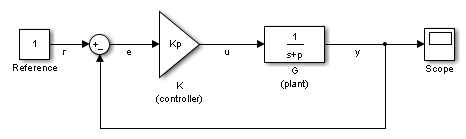
Obtain the closed-loop transfer function from the reference signal, r, to the plant output, y, for the ex_scd_simple_fdbk model.

Open the ex_scd_simple_fdbk model.

mdl = 'ex_scd_simple_fdbk';
open_system(mdl);

In this model:

Create an slLinearizer interface for the model.

sllin = slLinearizer(mdl);

To obtain the closed-loop transfer function from the reference signal, r, to the plant output, y, add both points to sllin.

addPoint(sllin,{'r','y'});

Obtain the closed-loop transfer function from r to y.

sys = getIOTransfer(sllin,'r','y');
tf(sys)

ans =
 
  From input "r" to output "y":
    3
  -----
  s + 8
 
Continuous-time transfer function.

The software adds a linearization input at r, dr, and a linearization output at y.

sys is the transfer function from dr to y, which is equal to .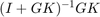

Specify Temporary Loop Opening to Get Plant Model

Obtain the plant model transfer function, G, for the ex_scd_simple_fdbk model.

Open the ex_scd_simple_fdbk model.

mdl = 'ex_scd_simple_fdbk';
open_system(mdl);

In this model:

Create an slLinearizer interface for the model.

sllin = slLinearizer(mdl);

To obtain the plant model transfer function, use u as the input point and y as the output point. To eliminate the effects of feedback, you must break the loop. You can break the loop at u, e, or y. For this example, break the loop at u. Add these points to sllin.

addPoint(sllin,{'u','y'});

Obtain the plant model transfer function.

sys = getIOTransfer(sllin,'u','y','u');
tf(sys)

ans =
 
  From input "u" to output "y":
    1
  -----
  s + 5
 
Continuous-time transfer function.

The second input argument specifies u as the input, while the fourth input argument specifies u as a temporary loop opening.

sys is the transfer function from du to y, which is equal to .

Obtain Open-Loop Response Transfer Function for Specific Parameter Combination

Suppose you batch linearize the scdcascade model for multiple transfer functions. For most linearizations, you vary the proportional (Kp2) and integral gain (Ki2) of the C2 controller in the 10% range. For this example, calculate the open-loop response transfer function for the inner loop, from e2 to y2, for the maximum value of Kp2 and Ki2.

Open the scdcascade model.

mdl = 'scdcascade';
open_system(mdl)

Create an slLinearizer interface for the model.

sllin = slLinearizer(mdl);

Vary the proportional (Kp2) and integral gain (Ki2) of the C2 controller in the 10% range.

Kp2_range = linspace(0.9*Kp2,1.1*Kp2,3);
Ki2_range = linspace(0.9*Ki2,1.1*Ki2,5);

[Kp2_grid,Ki2_grid] = ndgrid(Kp2_range,Ki2_range);

params(1).Name = 'Kp2';
params(1).Value = Kp2_grid;

params(2).Name = 'Ki2';
params(2).Value = Ki2_grid;

sllin.Parameters = params;

To calculate the open-loop transfer function for the inner loop, use e2 and y2 as analysis points. To eliminate the effects of the outer loop, break the loop at e2. Add e2 and y2 to sllin as analysis points.

addPoint(sllin,{'e2','y2'})

Determine the index for the maximum values of Ki2 and Kp2.

mdl_index = params(1).Value == max(Kp2_range) & params(2).Value == max(Ki2_range);

Obtain the open-loop transfer function from e2 to y2.

sys = getIOTransfer(sllin,'e2','y2','e2',mdl_index);

Obtain Offsets from Input/Output Transfer Function

Open Simulink model.

mdl = 'scdcascade';
open_system(mdl)

Create a linearization option set, and set the StoreOffsets option.

opt = linearizeOptions('StoreOffsets',true);

Create slLinearizer interface.

sllin = slLinearizer(mdl,opt);

Add analysis points to calculate the closed-loop transfer function.

addPoint(sllin,{'r','y1m'});

Calculate the input/output transfer function, and obtain the corresponding linearization offsets.

[sys,info] = getIOTransfer(sllin,'r','y1m');

View offsets.

info.Offsets

ans = 

  struct with fields:

             x: [6x1 double]
            dx: [6x1 double]
             u: 1
             y: 0
     StateName: {6x1 cell}
     InputName: {'r'}
    OutputName: {'y1m'}
            Ts: 0

Input Arguments

s — Interface to Simulink^® model

slLinearizer interface | slTuner interface

Interface to a Simulink model, specified as either an slLinearizer interface or an slTuner interface.

in — Input analysis point signal name

character vector | string | cell array of character vectors | string array

Input analysis point signal name, specified as:

• Character vector or string — Analysis point signal name.

  To determine the signal name associated with an analysis point, type s. The software displays the contents of s in the MATLAB^® command window, including the analysis point signal names, block names, and port numbers. Suppose that an analysis point does not have a signal name, but only a block name and port number. You can specify in as the block name. To use a point not in the list of analysis points for s, first add the point using addPoint.

  You can specify in as a uniquely matching portion of the full signal name or block name. Suppose that the full signal name of an analysis point is 'LoadTorque'. You can specify in as 'Torque' as long as 'Torque' is not a portion of the signal name for any other analysis point of s.

  For example, in = 'y1m'.

• Cell array of character vectors or string array — Specifies multiple analysis point names. For example, in = {'y1m','y2m'}.

out — Output analysis point signal name

character vector | string | cell array of character vectors | string array

Output analysis point signal name, specified as:

• Character vector or string — Analysis point signal name.

  To determine the signal name associated with an analysis point, type s. The software displays the contents of s in the MATLAB command window, including the analysis point signal names, block names, and port numbers. Suppose that an analysis point does not have a signal name, but only a block name and port number. You can specify out as the block name. To use a point not in the list of analysis points for s, first add the point using addPoint.

  You can specify out as a uniquely matching portion of the full signal name or block name. Suppose that the full signal name of an analysis point is 'LoadTorque'. You can specify out as 'Torque' as long as 'Torque' is not a portion of the signal name for any other analysis point of s.

  For example, out = 'y1m'.

• Cell array of character vectors or string array — Specifies multiple analysis point names. For example, out = {'y1m','y2m'}.

temp_opening — Temporary opening signal name

character vector | string | cell array of character vectors | string array

Temporary opening signal name, specified as:

• Character vector or string — Analysis point signal name.

  temp_opening must specify an analysis point that is in the list of analysis points for s. To determine the signal name associated with an analysis point, type s. The software displays the contents of s in the MATLAB command window, including the analysis point signal names, block names, and port numbers. Suppose that an analysis point does not have a signal name, but only a block name and port number. You can specify temp_opening as the block name. To use a point not in the list of analysis points for s, first add the point using addPoint.

  You can specify temp_opening as a uniquely matching portion of the full signal name or block name. Suppose that the full signal name of an analysis point is 'LoadTorque'. You can specify temp_opening as 'Torque' as long as 'Torque' is not a portion of the signal name for any other analysis point of s.

  For example, temp_opening = 'y1m'.

• Cell array of character vectors or string array — Specifies multiple analysis point names. For example, temp_opening = {'y1m','y2m'}.

ios — Linearization I/Os

linearization I/O object

Linearization I/Os, created using linio, specified as a linearization I/O object.

ios must specify signals that are in the list of analysis points for s. To view the list of analysis points, type s. To use a point that is not in the list of analysis points for s, you must first add the point to the list using addPoint.

For example:

ios(1) = linio('scdcascade/setpoint',1,'input');
ios(2) = linio('scdcascade/Sum',1,'output');

Here, ios(1) specifies an input, and ios(2) specifies an output.

mdl_index — Index for linearizations of interest

array of logical values | vector of positive integers

Index for linearizations of interest, specified as:

• Array of logical values — Logical array index of linearizations of interest. Suppose that you vary two parameters, par1 and par2, and want to extract the linearization for the combination of par1 > 0.5 and par2 <= 5. Use:

  params = s.Parameters;
  mdl_index = params(1).Value>0.5 & params(2).Value <= 5;

  The expression params(1).Value>0.5 & params(2).Value<5 uses logical indexing and returns a logical array. This logical array is the same size as params(1).Value and params(2).Value. Each entry contains the logical evaluation of the expression for corresponding entries in params(1).Value and params(2).Value.

• Vector of positive integers — Linear index of linearizations of interest. Suppose that you vary two parameters, par1 and par2, and want to extract the linearization for the combination of par1 > 0.5 and par2 <= 5. Use:

  params = s.Parameters;
  mdl_index = find(params(1).Value>0.5 & params(2).Value <= 5);

  The expression params(1).Value>0.5 & params(2).Value<5 returns a logical array. find returns the linear index of every true entry in the logical array

Output Arguments

linsys — Transfer function for specified I/Os

state-space model

Transfer function for specified I/Os, returned as described in the following:

• If you did not configure s.Parameters and s.OperatingPoints, the software calculates linsys using the default model parameter values. The software uses the model initial conditions as the linearization operating point. linsys is returned as a state-space model.

• If you configured s.Parameters only, the software computes a linearization for each parameter grid point. linsys is returned as a state-space model array of the same size as the parameter grid.

• If you configured s.OperatingPoints only, the software computes a linearization for each specified operating point. linsys is returned as a state-space model array of the same size as s.OperatingPoints.

• If you configured s.Parameters and specified s.OperatingPoints as a single operating point, the software computes a linearization for each parameter grid point. The software uses the specified operating point as the linearization operating point. linsys is returned as a state-space model array of the same size as the parameter grid.

• If you configured s.Parameters and specified s.OperatingPoints as multiple operating point objects, the software computes a linearization for each parameter grid point. The software requires that s.OperatingPoints is the same size as the parameter grid specified by s.Parameters. The software computes each linearization using corresponding operating points and parameter grid points. linsys is returned as a state-space model array of the same size as the parameter grid.

• If you configured s.Parameters and specified s.OperatingPoints as multiple simulation snapshot times, the software simulates and linearizes the model for each snapshot time and parameter grid point combination. Suppose that you specify a parameter grid of size p and N snapshot times. linsys is returned as a state-space model array of size N-by-p.

For most models, linsys is returned as an ss object or an array of ss objects. However, if your model contains one of the following blocks in the linearization path defined by in and out, then linsys returns the specified type of state-space model.

Block	linsys Type
Block with a substitution specified as a genss object or tunable model object	genss
Block with a substitution specified as an uncertain model, such as uss	uss (Robust Control Toolbox)
Sparse Second Order block	mechss
Descriptor State-Space block configured to linearize to a sparse model	sparss

info — Linearization information

structure

Linearization information, returned as a structure with the following fields:

Offsets — Linearization offsets

[] (default) | structure | structure array

Linearization offsets, returned as [] if s.Options.StoreOffsets is false. Otherwise, Offsets is returned as one of the following:

• If linsys is a single state-space model, then Offsets is a structure.

• If linsys is an array of state-space models, then Offsets is a structure array with the same dimensions as linsys.

Each offset structure has the following fields:

Field	Description
x	State offsets used for linearization, returned as a column vector of length nx, where nx is the number of states in linsys.
y	Output offsets used for linearization, returned as a column vector of length ny, where ny is the number of outputs in linsys.
u	Input offsets used for linearization, returned as a column vector of length nu, where nu is the number of inputs in linsys.
dx	Derivative offsets for continuous time systems or updated state values for discrete-time systems, returned as a column vector of length nx.
StateName	State names, returned as a cell array that contains nx elements that match the names in linsys.StateName.
InputName	Input names, returned as a cell array that contains nu elements that match the names in linsys.InputName.
OutputName	Output names, returned as a cell array that contains ny elements that match the names in linsys.OutputName.
Ts	Sample time of the linearized system, returned as a scalar that matches the sample time in linsys.Ts. For continuous-time systems, Ts is 0.

If Offsets is a structure array, you can configure an LPV System block using the offsets. To do so, first convert them to the required format using getOffsetsForLPV. For an example, see Approximate Nonlinear Behavior Using Array of LTI Systems.

Advisor — Linearization diagnostic information

[] (default) | LinearizationAdvisor object | array of LinearizationAdvisor objects

Linearization diagnostic information, returned as [] if s.Options.StoreAdvisor is false. Otherwise, Advisor is returned as one of the following:

• If linsys is a single state-space model, Advisor is a LinearizationAdvisor object.

• If linsys is an array of state-space models, Advisor is an array of LinearizationAdvisor objects with the same dimensions as linsys.

LinearizationAdvisor objects store linearization diagnostic information for individual linearized blocks. For an example of troubleshooting linearization results using a LinearizationAdvisor object, see Troubleshoot Linearization Results at Command Line.

More About

Transfer Functions

A transfer function is an LTI system response at a linearization output point to a linearization input. You perform linear analysis on transfer functions to understand the stability, time-domain characteristics, or frequency-domain characteristics of a system.

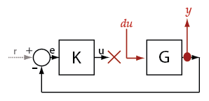
You can calculate multiple transfer functions for a given block diagram. Consider the ex_scd_simple_fdbk model:

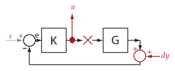
You can calculate the transfer function from the reference input signal to the plant output signal. The reference input (also referred to as setpoint), r, originates at the Reference block, and the plant output, y, originates at the G block. This transfer function is also called the overall closed-loop transfer function. To calculate this transfer function, the software adds a linearization input at r, dr, and a linearization output at y.

The software calculates the overall closed-loop transfer function as the transfer function from dr to y, which is equal to (I+GK)^-1GK.

Observe that the transfer function from r to y is equal to the transfer function from dr to y.

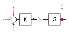
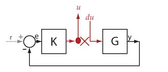
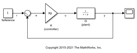
You can calculate the plant transfer function from the plant input, u, to the plant output, y. To isolate the plant dynamics from the effects of the feedback loop, introduce a loop break (or opening) at y, e, or, as shown, at u.

The software breaks the loop and adds a linearization input, du, at u, and a linearization output at y. The plant transfer function is equal to the transfer function from du to y, which is G.

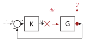
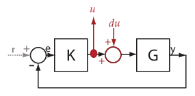
Similarly, to obtain the controller transfer function, calculate the transfer function from the controller input, e, to the controller output, u. Break the feedback loop at y, e, or u.

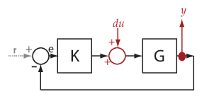
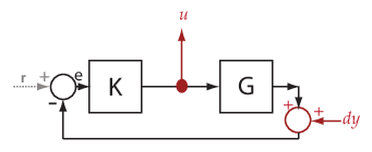
You can use getIOTransfer to obtain various open-loop and closed-loop transfer functions. To configure the transfer function, specify analysis points as inputs, outputs, and openings (temporary or permanent), in any combination. The software treats each combination uniquely. Consider the following code that shows some different ways that you can use the analysis point, u, to obtain a transfer function:

sllin = slLinearizer('ex_scd_simple_fdbk')

addPoint(sllin,{'u','e','y'})

T0 = getIOTransfer(sllin,'e','y','u');
T1 = getIOTransfer(sllin,'u','y');
T2 = getIOTransfer(sllin,'u','y','u');
T3 = getIOTransfer(sllin,'y','u');
T4 = getIOTransfer(sllin,'y','u','u');
T5 = getIOTransfer(sllin,'u','u'); 
T6 = getIOTransfer(sllin,'u','u','u');

In T0, u specifies a loop break. In T1, u specifies only an input, whereas in T2, u specifies an input and an opening, also referred to as an open-loop input. In T3, u specifies only an output, whereas in T4, u specifies an output and an opening, also referred to as an open-loop output. In T5, u specifies an input and an output, also referred to as a complementary sensitivity point. In T6, u specifies an input, an output, and an opening, also referred to as a loop transfer point. The table describes how getIOTransfer treats the analysis points, with an emphasis on the different uses of u.

u Specifies...	How getIOTransfer Treats Analysis Points	Transfer Function
Loop break Example code: T0 = getIOTransfer(... sllin,'e','y','u')	The software stops the signal flow at u, adds a linearization input, de, at e, and a linearization output at y. Since there is not path from de to e, the transfer function is zero.	$$\begin{array}{l}\begin{array}{l}y=G0\hfill \\ \to y=0\hfill \end{array}\\ \therefore T_0=0\end{array}$$
Input Example code: T1 = getIOTransfer(... sllin,'u','y')	The software adds a linearization input, du, at u, and a linearization output at y.	$$\begin{array}{l}y=G\left(du-Ky\right)\\ \to y=Gdu-GKy\\ \to \left(I+GK\right)y=Gdu\\ \to y={\left(I+GK\right)}^{-1}Gdu\\ \therefore T_1={\left(I+GK\right)}^{-1}G\end{array}$$
Open-loop input Example code: T2 = getIOTransfer(... sllin,'u','y','u')	The software breaks the signal flow and adds a linearization input, du, at u, and a linearization output at y.	$$\begin{array}{l}y=G\left(du+0\right)\hfill \\ \begin{array}{l}\to y=Gdu\\ \therefore T_2=G\end{array}\hfill \end{array}$$
Output Example code: T3 = getIOTransfer(... sllin,'y','u')	The software adds a linearization input, dy, at y and a linearization output at u.	$$\begin{array}{l}u=-K\left(dy+Gu\right)\\ \to u=-Kdy-KGu\\ \to \left(I+KG\right)u=-Kdy\\ \to u=-{\left(I+KG\right)}^{-1}Kdy\\ \therefore T_3=-{\left(I+KG\right)}^{-1}K\end{array}$$
Open-loop output Example code: T4 = getIOTransfer(... sllin,'y','u','u')	The software adds a linearization input, dy, at y and adds a linearization output and breaks the signal flow at u.	$$\begin{array}{l}u=-K\left(dy+G0\right)\hfill \\ \begin{array}{l}\to u=-Kdy\\ \therefore T_4=-K\end{array}\hfill \end{array}$$
Complementary sensitivity point Example code: T5 = getIOTransfer(... sllin,'u','u') Tip You also can obtain the complementary sensitivity function using getCompSensitivity.	The software adds a linearization output and a linearization input, du, at u.	$$\begin{array}{l}u=-KG\left(du+u\right)\hfill \\ \to u=-KGdu-KGu\hfill \\ \to \left(I+KG\right)u=-KGdu\hfill \\ \begin{array}{l}\to u=-{\left(I+KG\right)}^{-1}KGdu\\ \therefore T_5=-{\left(I+KG\right)}^{-1}KG\end{array}\hfill \end{array}$$
Loop transfer function point Example code: T6 = getIOTransfer(... sllin,'u','u','u') Tip You also can obtain the loop transfer function using getLoopTransfer.	The software adds a linearization output, breaks the loop, and adds a linearization input, du, at u.	$$\begin{array}{l}u=-KG\left(du+0\right)\\ \to u=-KGdu\\ \therefore T_6=-KG\end{array}$$

The software does not modify the Simulink model when it computes the transfer function.

Analysis Points

Analysis points, used by the slLinearizer and slTuner interfaces, identify locations within a model that are relevant for linear analysis and control system tuning. You use analysis points as inputs to the linearization commands, such as getIOTransfer, getLoopTransfer, getSensitivity, and getCompSensitivity. As inputs to the linearization commands, analysis points can specify any open-loop or closed-loop transfer function in a model. You can also use analysis points to specify design requirements when tuning control systems using commands such as systune.

Location refers to a specific block output port within a model or to a bus element in such an output port. For convenience, you can use the name of the signal that originates from this port to refer to an analysis point.

You can add analysis points to an slLinearizer or slTuner interface, s, when you create the interface. For example:

s = slLinearizer('scdcascade',{'u1','y1'});

Alternatively, you can use the addPoint command.

To view all the analysis points of s, type s at the command prompt to display the interface contents. For each analysis point of s, the display includes the block name and port number and the name of the signal that originates at this point. You can also programmatically obtain a list of all the analysis points using getPoints.

For more information about how you can use analysis points, see Mark Signals of Interest for Control System Analysis and Design and Mark Signals of Interest for Batch Linearization.

Permanent Openings

Permanent openings, used by the slLinearizer and slTuner interfaces, identify locations within a model where the software breaks the signal flow. The software enforces these openings for linearization and tuning. Use permanent openings to isolate a specific model component. Suppose that you have a large-scale model capturing aircraft dynamics and you want to perform linear analysis on the airframe only. You can use permanent openings to exclude all other components of the model. Another example is when you have cascaded loops within your model and you want to analyze a specific loop.

Location refers to a specific block output port within a model. For convenience, you can use the name of the signal that originates from this port to refer to an opening.

You can add permanent openings to an slLinearizer or slTuner interface, s, when you create the interface or by using the addOpening command. To remove a location from the list of permanent openings, use the removeOpening command.

To view all the openings of s, type s at the command prompt to display the interface contents. For each permanent opening of s, the display includes the block name and port number and the name of the signal that originates at this location. You can also programmatically obtain a list of all the permanent loop openings using getOpenings.

Version History

Introduced in R2013b

R2020b: Linearize Simulink model to a sparse state-space model

You can linearize and obtain a sparse model from a Simulink model that contains a Sparse Second Order or Descriptor State-Space block.

• mechss model when you use a Sparse Second Order in your Simulink model.

• sparss model when you use a Descriptor State-Space block and select the Linearize to sparse model block parameter.

For more information, see Sparse Model Basics. For an example, see Linearize Simulink Model to a Sparse Second-Order Model Object.

R2016b: Compute operating point offsets for model inputs, outputs, states, and state derivatives during linearization

You can compute operating point offsets for model inputs, outputs, states, and state derivatives when linearizing Simulink models. Thee offsets streamline the creation of linear parameter-varying (LPV) systems.

To obtain operating point offsets, first create a linearizeOptions or slTunerOptions object and set the StoreOffsets option to true. Then, create an slLinearizer or slTuner interface for the model.

You can extract the offsets from the info output argument of getIOTransfer and convert them into the required format for the LPV System block using the getOffsetsForLPV function.