Troubleshoot Linearization Results at Command Line
This example shows how to debug the linearization of a Simulink® model at the command line using a LinearizationAdvisor object. You can also troubleshoot linearization results interactively. For more information, see Troubleshoot Linearization Results in Model Linearizer.
Open the model.
mdl = 'scdpendulum';
open_system(mdl)
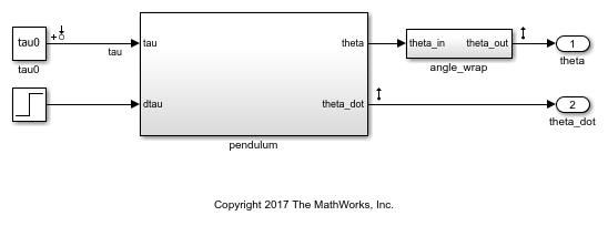
The initial condition for the pendulum angle is 90 degrees counterclockwise from the upright unstable equilibrium of 0 degrees. The initial condition for the pendulum angular velocity is 0 deg/s. The nominal torque to maintain this state is -49.05 N m. This configuration is saved as the model initial condition.
Linearize the Model
Linearize the model using the analysis points defined in the model and the model operating point.
io = getlinio(mdl);
linsys = linearize(mdl,io);
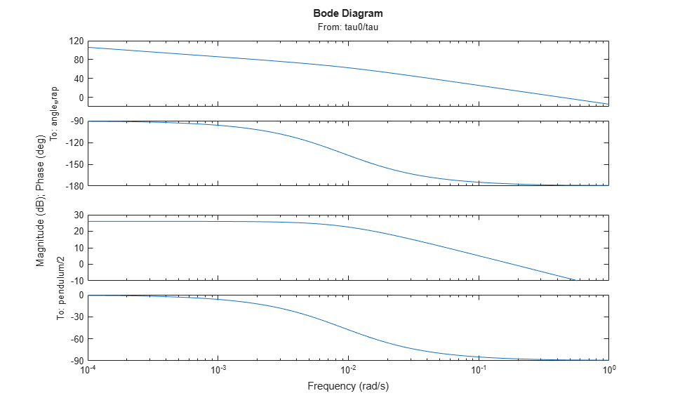
To check the linearization result, plot its Bode response.
bode(linsys)
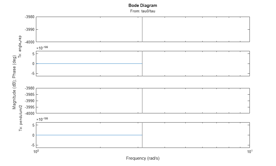
The model linearized to zero such that the torque, tau, has no effect on the angle or angular velocity. To find the source of the zero linearization, you can use a LinearizationAdvisor object.
Linearize Model with Advisor Enabled
To collect diagnostic information during linearization and create an advisor for troubleshooting, first create a linearizeOptions option set, specifying the StoreAdvisor option as true.
opt = linearizeOptions('StoreAdvisor',true);
Linearize the Simulink model using this option set. Return the info output argument, which contains linearization diagnostic information in a LinearizationAdvisor object.
[linsys1,~,info] = linearize(mdl,io,opt);
Extract the LinearizationAdvisor object.
advisor = info.Advisor;
Highlight Linearization Path
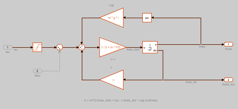
To show the linearization path for the current linearization, use highlight.
highlight(advisor)
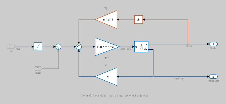
View the pendulum subsystem.
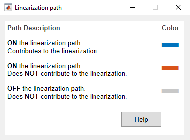
As shown in the Linearization path dialog box, the blocks highlighted in:
Blue numerically influence the model linearization.
Red are on the linearization path but do not influence the model linearization for the current operating point and block parameters.
Since the model linearized to zero, there are no blocks that contribute to the linearization.
Investigate Potentially Problematic Blocks
To obtain diagnostic information for blocks that may be problematic for linearization, use advise. This function returns a new LinearizationAdvisor object that contains information on blocks on the linearization path that satisfy at least one of the following criteria:
Have diagnostic messages regarding their linearization
Linearize to zero
Have substituted linearizations
adv1 = advise(advisor);
View a summary of the diagnostic information for these blocks, use getBlockInfo.
getBlockInfo(adv1)
ans =

Linearization Diagnostics for the Blocks:

Block Info:
-----------
Index   BlockPath                                           Is On Path   Contributes To Linearization   Linearization Method
1.      scdpendulum/pendulum/Saturation                     Yes          No                             Exact
2.      scdpendulum/angle_wrap/Trigonometric Function1      Yes          No                             Perturbation
3.      scdpendulum/pendulum/Trigonometric Function         Yes          No                             Perturbation
In this case, the advisor reports three potentially problematic blocks, a Saturation block and two Trigonometric Function blocks. When you run this example in MATLAB®, the block paths display as hyperlinks. To go to one of these blocks in the model, click the corresponding block path hyperlink.
To view more information about a specific block linearization, use getBlockInfo. For information on the available diagnostics, see BlockDiagnostic.
For example, obtain the diagnostic information for the Saturation block.
diagInfo = getBlockInfo(adv1,1)
diagInfo =

Linearization Diagnostics for scdpendulum/pendulum/Saturation with properties:

                      IsOnPath: 'Yes'
    ContributesToLinearization: 'No'
           LinearizationMethod: 'Exact'
                 Linearization: [1×1 ss]
                OperatingPoint: [1×1 linearize.advisor.BlockOperatingPoint]
This block has the following two diagnostic messages regarding its linearization result.
The block is analytically linearized to zero because the signal input value (-49.05) is outside the lower limit of the block (-49). Consider linearizing the block as a gain.
The linearization of the block has at least one zero input/output pair resulting in a zero input/output pair for the system linearization. Modify the block parameters and/or operating point if the block is expected to contribute to the model linearization.
The first message indicates that the block is linearized outside of its lower saturation limit of -49, since the input operating point is -49.05.
The message also indicates that the block can be linearized as a gain, which linearizes the block as 1 regardless of the input operating point.
When you run this example in MATLAB, the text linearizing the block as a gain displays as a hyperlink. To open the Block Parameters dialog box for the Saturation block, and highlight the option for linearizing the block as a gain, click this hyperlink.
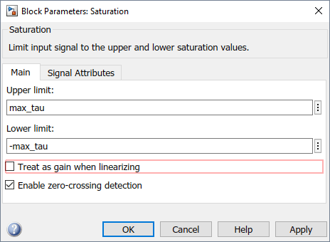
Select Treat as gain when linearizing, and click OK.
Alternatively, you can set this parameter from the command line.
set_param('scdpendulum/pendulum/Saturation','LinearizeAsGain','on')
The second diagnostic message states that the linearization of this block causes the overall model to linearize to zero. View the linearization of this block.
diagInfo.Linearization
ans =

  D =
       u1
   y1   0

Name: Saturation
Static gain with offsets.
Since this block linearized to zero, modifying the block linearization by treating it as a gain is a good first step toward obtaining a nonzero model linearization.
Relinearize Model
To see the effect of treating the Saturation block as a gain, relinearize the model, and plot its Bode response.
[linsys2,~,info] = linearize(mdl,io,opt);
bode(linsys2)
The model linearization is now nonzero.
To check if any blocks are still potentially problematic for linearization, extract the advisor object, and use the advise function.
advisor2 = info.Advisor;
adv2 = advise(advisor2);
View the block diagnostic information.
getBlockInfo(adv2)
ans =

Linearization Diagnostics for the Blocks:

Block Info:
-----------
Index   BlockPath                                           Is On Path   Contributes To Linearization   Linearization Method
1.      scdpendulum/angle_wrap/Trigonometric Function1      Yes          No                             Perturbation
2.      scdpendulum/pendulum/Trigonometric Function         Yes          No                             Perturbation
The two Trigonometric Function blocks are still listed.
Highlight the linearization path for the updated linearization.
highlight(advisor2)
View the pendulum subsystem.
To understand why these blocks are not contributing to the linearization, view their corresponding block diagnostic information. For example, obtain the diagnostic information for the second Trigonometric Function block.
diagInfo = getBlockInfo(adv2,2)
diagInfo =

Linearization Diagnostics for scdpendulum/pendulum/Trigonometric Function with properties:

                      IsOnPath: 'Yes'
    ContributesToLinearization: 'No'
           LinearizationMethod: 'Perturbation'
                 Linearization: [1×1 ss]
                OperatingPoint: [1×1 linearize.advisor.BlockOperatingPoint]
View the linearization of this block.
diagInfo.Linearization
ans =

  D =
       u1
   y1   0

Name: Trigonometric
Function
Static gain with offsets.
The block linearized to zero. To see if this result is expected for the current operating condition of the block, check its operating point.
diagInfo.OperatingPoint
ans =

Block Operating Point for scdpendulum/pendulum/Trigonometric Function


Inputs:
-------
Port   u
1      1.5708
The input operating point of the block is  .
.
You can find the linearization of the block analytically by taking the first derivative of the sin function with respect to the input.
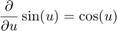
Therefore, when evaluated at  the linearization of the block is zero. The source of the input is the first output of the second-order integrator, which is dependent upon the state
 theta. Therefore, this block linearizes to zero if  , where
  is an integer. The same condition applies for the other Trigonometric Function block in the angle_wrap subsystem. If these blocks are not expected to linearize to zero, you can modify the operating point state
 theta, and relinearize the model.
Create and Run Custom Queries
The Linearization Advisor also provides objects and functions for creating custom queries. Using these queries, you can find blocks in your model that match specific criteria. For example, to find all SISO blocks that are linearized using numerical perturbation, first create query objects for each search criterion:
Has one input
Has one output
Is numerically perturbed
qIn = linqueryHasInputs(1);
qOut = linqueryHasOutputs(1);
qPerturb = linqueryIsNumericallyPerturbed;
Create a CompoundQuery object by combining these query objects using logical operators.
sisopert = qIn & qOut & qPerturb;
Search the block diagnostics in advisor2 for blocks matching these criteria.
sisopertBlocks = find(advisor2,sisopert)
sisopertBlocks =

  LinearizationAdvisor with properties:

               Model: 'scdpendulum'
      OperatingPoint: [1×1 opcond.OperatingPoint]
    BlockDiagnostics: [3×1 linearize.advisor.BlockDiagnostic]
           QueryType: '((Has 1 Inputs & Has 1 Outputs) & Perturbation)'
There are three SISO blocks in the model that are linearized using numerical perturbation.
For more information on using custom queries, see Find Blocks in Linearization Results Matching Specific Criteria.
bdclose(mdl)