findop
Find steady-state operating point from specifications (trimming) or simulation
Syntax
Description
op = findop(mdl,opspec)opspec. Typically, you trim the model at a steady-state operating
point. The Simulink® model must be open. If opspec is an array of
operating point specifications, findop returns an array of
corresponding operating points.
Examples
Open the Simulink model.
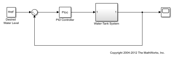
mdl = 'watertank';
open_system(mdl)

Trim the model to find a steady-state operating point where the water tank level is 10.
Create default operating point specification object.
opspec = operspec(mdl);
Configure specifications for the first model state. The first state must be at steady state with a lower bound of 0. Provide an initial guess of 2 for the state value.
opspec.States(1).SteadyState = 1;
opspec.States(1).x = 2;
opspec.States(1).Min = 0;
Configure the second model state as a known state with a value of 10.
opspec.States(2).Known = 1;
opspec.States(2).x = 10;
Find the operating point that meets these specifications.
op = findop(mdl,opspec);
 Operating point search report:
---------------------------------

opreport =


 Operating point search report for the Model watertank.
 (Time-Varying Components Evaluated at time t=0)

Operating point search completed successfully using optimization.
States:
----------
 Min     x     Max   dxMin    dx   dxMax
______ ______ ______ ______ ______ ______

(1.) watertank/PID Controller/Integrator/Continuous/Integrator
  0    1.2649  Inf     0      0      0
(2.) watertank/Water-Tank System/H
  10     10     10     0      0      0

Inputs: None
----------

Outputs: None
----------
Open the Simulink model.
mdl = 'watertank';
open_system(mdl)

Vary parameters A and b within 10% of their nominal values, and create a 3-by-4 parameter grid.
[A_grid,b_grid] = ndgrid(linspace(0.9*A,1.1*A,3),...
                         linspace(0.9*b,1.1*b,4));
Create a parameter structure array, specifying the name and grid points for each parameter.
params(1).Name = 'A';
params(1).Value = A_grid;
params(2).Name = 'b';
params(2).Value = b_grid;
Create a default operating point specification for the model.
opspec = operspec(mdl);
Trim the model using the specified operating point specification and parameter grid.
opt = findopOptions('DisplayReport','off');
op = findop(mdl,opspec,params,opt);
op is a 3-by-4 array of operating point objects that correspond to the specified parameter grid points.
Open the Simulink model.
mdl = 'watertank';
open_system(mdl)

Create a default operating point specification object.
opspec = operspec(mdl);
Create an option set that sets the optimizer type to gradient descent and suppresses the search report display.
opt = findopOptions('OptimizerType','graddescent','DisplayReport','off');
Trim the model using the specified option set.
op = findop(mdl,opspec,opt);
Open the Simulink model.
mdl = 'watertank';
open_system(mdl)
Create default operating point specification object.
opspec = operspec(mdl);
Configure specifications for the first model state.
opspec.States(1).SteadyState = 1;
opspec.States(1).x = 2;
opspec.States(1).Min = 0;
Configure specifications for the second model state.
opspec.States(2).Known = 1;
opspec.States(2).x = 10;
Find the operating point that meets these specifications, and return the operating point search report. Create an option set to suppress the search report display.
opt = findopOptions('DisplayReport',false);
[op,opreport] = findop(mdl,opspec,opt);
opreport describes how closely the optimization algorithm met the specifications at the end of the operating point search.
opreport
opreport =


 Operating point search report for the Model watertank.
 (Time-Varying Components Evaluated at time t=0)

Operating point search completed successfully using optimization.
States:
----------
 Min     x     Max   dxMin    dx   dxMax
______ ______ ______ ______ ______ ______

(1.) watertank/PID Controller/Integrator/Continuous/Integrator
  0    1.2649  Inf     0      0      0
(2.) watertank/Water-Tank System/H
  10     10     10     0      0      0

Inputs: None
----------

Outputs: None
----------
dx is the time derivative for each state. Since all dx values are zero, the operating point is at steady state.
Open the Simulink model.
mdl = 'magball';
open_system(mdl)
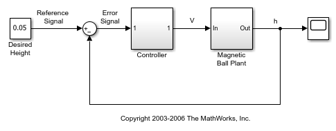
Simulate the model, and extract operating points at 10 and 20 time units.
op = findop(mdl,[10,20]);
op is a column vector of operating points, with one element for each snapshot time.
Display the first operating point.
op(1)
ans =


 Operating point for the Model magball.
 (Time-Varying Components Evaluated at time t=10)

States:
----------
    x
__________

(1.) magball/Controller/PID Controller/Filter/Cont. Filter/Filter
5.4732e-07
(2.) magball/Controller/PID Controller/Integrator/Continuous/Integrator
 14.0071
(3.) magball/Magnetic Ball Plant/Current
  7.0036
(4.) magball/Magnetic Ball Plant/dhdt
8.443e-08
(5.) magball/Magnetic Ball Plant/height
   0.05

Inputs: None
----------
Open Simulink model.
mdl = 'watertank';
open_system(mdl)

Specify parameter values. The parameter grids are 5-by-4 arrays.
[A_grid,b_grid] = ndgrid(linspace(0.9*A,1.1*A,5),...
                         linspace(0.9*b,1.1*b,4));
params(1).Name = 'A';
params(1).Value = A_grid;
params(2).Name = 'b';
params(2).Value = b_grid;
Simulate the model and extract operating points at 0, 5, and 10 time units.
op = findop(mdl,[0 5 10],params);
findop simulates the model for each parameter value combination, and extracts operating points at the specified simulation times.
op is a 3-by-5-by-4 array of operating point objects.
size(op)
ans =

     3     5     4
Input Arguments
Output Arguments
More About
Tips
You can initialize an operating point search at a simulation snapshot or a previously computed operating point using
initopspec.Linearize the model at the operating point
opusinglinearize.To extract state and input values from an operating point object, use
getstatestructandgetinputstruct, respectively.
Algorithms
By default, findop uses the optimizer
graddescent-elim. To use a different optimizer, change the value
of OptimizerType in options using findopOptions.
findop automatically sets these Simulink model
properties for optimization:
BufferReuse = "off"BlockReductionOpt = 'off"SaveFormat = "StructureWithTime"
After the optimization completes, Simulink restores the original model properties.
Alternative Functionality
App
As an alternative to the findop command, you can find
operating points in one of the following ways.
Compute operating points using the Steady State Manager. For an example, see Compute Operating Points from Specifications Using Steady State Manager.
If you are computing an operating point for linearization, you can find the operating point and linearize the model using the Model Linearizer. For an example, see Compute Operating Points from Specifications Using Model Linearizer.