frest.simView
Namespace: frest
Plot frequency response model in time- and frequency-domain
Syntax
frest.simView(simout,input,sysest)

frest.simView(simout,input,sysest,sys)
Description
frest.simView(
opens the Simulation Results Viewer and plots the following frequency response estimation results:simout,input,sysest)
Time-domain simulation
simoutof the Simulink modelFFT of time-domain simulation
simoutBode of estimated system
sysestThis Bode plot is available when you create the input signal using
frest.Sinestreamorfrest.Chirp. In this plot, you can interactively select frequencies or a frequency range for viewing the results in all three plots.
You obtain simout and sysest from the
frestimate command using the input signal
input.
frest.simView(
includes the linear system simout,input,sysest,sys)sys in the Bode plot when you create the input
signal using frest.Sinestream or frest.Chirp. Use
this syntax to compare the linear system to the frequency response estimation results.
Examples
The Simulation Results Viewer lets you examine the results of frequency response estimation frequency by frequency. You open the viewer using the frest.simView command. To do so, store the simulation data using the simout output argument of frestimate.
Estimate the open-loop response of the plant in the watertank model. First, open the model.
model = 'watertank';
open_system(model)
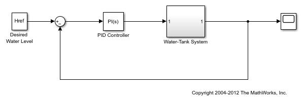
Define a linearization I/O set that specifies the plant, and find a steady-state operating point for estimation.
io(1)=linio('watertank/PID Controller',1,'input');
io(2)=linio('watertank/Water-Tank System',1,'openoutput');

watertank_spec = operspec(model);
opOpts = findopOptions('DisplayReport','off');
op = findop(model,watertank_spec,opOpts);
Then, create an input signal for estimation, and estimate the frequency response of the specified portion of the model. Use the simout output argument to store the estimation data.
input = frest.Sinestream('Frequency',logspace(-3,2,10));
[sysest,simout] = frestimate(model,op,io,input);
Open the Simulation Results Viewer.
frest.simView(simout,input,sysest)
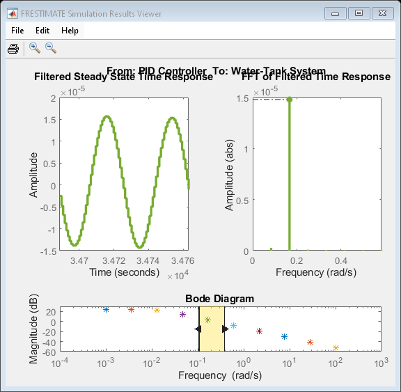
The viewer shows you the steady-state time response and the FFT of that response for all frequencies within the range you select on the Bode Diagram section of the viewer. These plots can help you identify when the response deviates from the expected response. For more information about using the Simulation Results Viewer, see Analyze Estimated Frequency Response.
If you have a linear model of the system you are estimating, you can use the model as a baseline response for comparison in the viewer. For instance, you can compare a model obtained by exact linearization to the estimated frequency response. Use the linearization I/O set and the operating point to compute an exact linearization of the watertank plant.
syslin = linearize(model,io,op);
Open the Simulation Results Viewer again, this time providing syslin as an input argument.
frest.simView(simout,input,sysest,syslin)
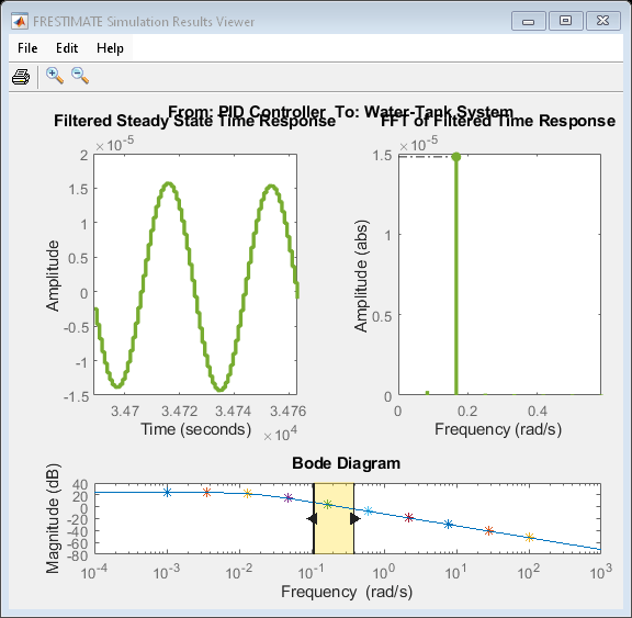
The Bode Diagram section of the viewer includes a line showing the exact response syslin. This view can be useful to identify particular frequencies where the estimated response deviates from the linearization.
Tips
Import Variables
After you estimate a new frequency response model, you can import the estimation results into the Simulation Results Viewer.
In the Simulation Results Viewer, select File > Import.
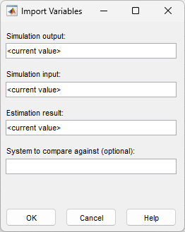
In the Import Variables dialog box, specify the names of variables available in the MATLAB® workspace for:
Simulation output — This output, obtained from the
frestimatecommand, appears in the time response plot and the FFT.Simulation input — Input signal used for estimation.
Estimation result — This result, obtained from the
frestimatecommand, appears in the Bode plot.System to compare against (optional) — Any linear system to appear in the Bode plot with the estimation result.
Tip
You can also import a new linear system to compare the existing estimation results by specifying only the variable for System to compare against (optional).
Version History
Introduced in R2009b