Discrete Wavelet Analysis
Wavelet Toolbox™ software enables you to analyze signals, images, and 3-D data using orthogonal and biorthogonal critically-sampled discrete wavelet analysis. Critically-sampled discrete wavelet analysis is also known as decimated discrete wavelet analysis. Decimated discrete wavelet analysis is most appropriate for data compression, denoising, and the sparse representation of certain classes of signals and images.
In decimated discrete wavelet analysis, the scales and translations are dyadic.
1-D Wavelet Denoising
This example shows how to denoise a signal using discrete wavelet analysis.
Create a reference signal.
len = 2^11;
h = [4  -5  3  -4  5  -4.2   2.1   4.3  -3.1   5.1  -4.2];
t = [0.1  0.13  0.15  0.23  0.25  0.40  0.44  0.65  0.76  0.78  0.81];
h  = abs(h);
w  = 0.01*[0.5 0.5 0.6 1 1 3 1 1 0.5 0.8 0.5];
tt = linspace(0,1,len);
xref = zeros(1,len);
for j=1:11
    xref = xref+(h(j)./(1+((tt-t(j))/w(j)).^4));
end
Add zero-mean white Gaussian noise with a variance of 0.25.
rng default
x = xref + 0.5*randn(size(xref));
plot(tt,x)
axis tight

Denoise the signal down to level 3 using the Daubechies least asymmetric wavelet with 4 vanishing moments. Use the universal threshold selection rule of Donoho and Johnstone with soft thresholding based on the DWT coefficients at level 1. Use the periodization signal extension mode — dwtmode('per'). Plot the result along with the reference signal for comparison.
origmode = dwtmode('status','nodisplay');
dwtmode('per','nodisplay')
xd = wdenoise(x,3,'Wavelet','sym4', ...
    'DenoisingMethod','UniversalThreshold','NoiseEstimate','LevelIndependent');
plot(tt,xd)
axis tight
hold on
plot(tt,xref,'r')
hold off
legend('Denoised','Reference')

Restore the original extension mode.
dwtmode(origmode,'nodisplay')2-D Decimated Discrete Wavelet Analysis
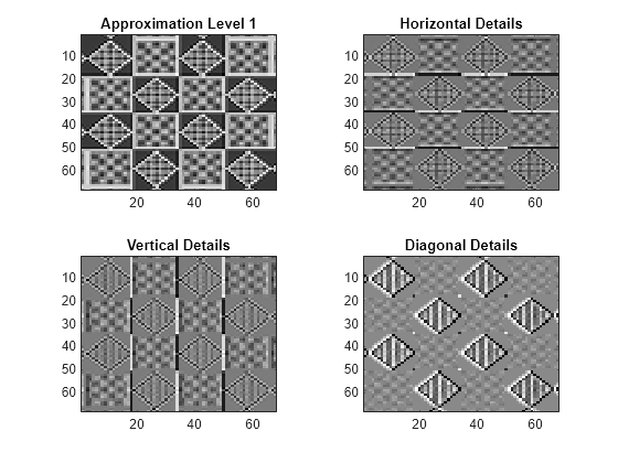
This example shows how to obtain the 2-D DWT of an input image.
Load and display the image. The image consists of vertical, horizontal, and diagonal patterns.
load tartan
imagesc(X)
colormap(gray)
Obtain the 2-D DWT at level 1 using the biorthogonal B-spline wavelet and scaling filters with 2 vanishing moments in the analysis filters and 4 vanishing moments in the synthesis filters.
[C,S] = wavedec2(X,1,'bior2.4');Extract the horizontal, vertical, and diagonal wavelet coefficients and the approximation coefficients.
[H,V,D] = detcoef2('all',C,S,1);
A = appcoef2(C,S,'bior2.4');
Display the results.
tiledlayout(2,2)
nexttile
imagesc(A)
title('Approximation Level 1')
colormap(gray)
nexttile
imagesc(H)
title('Horizontal Details')
nexttile
imagesc(V)
title('Vertical Details')
nexttile
imagesc(D)
title('Diagonal Details')

You see that the wavelet details are sensitive to particular orientations in the input image. The approximation coefficients are a lowpass approximation to the original image.
Nondecimated Discrete Wavelet Analysis
This example shows how to obtain the nondecimated (stationary) wavelet transform of a noisy frequency-modulated signal.
Load the noisy Doppler signal and obtain the stationary wavelet transform down to level 4.
load noisdopp
swc = swt(noisdopp,4,'sym8');
Plot the original signal and the level 1 and 3 wavelet coefficients. Plot the level 4 approximation.
tiledlayout('vertical')
nexttile
plot(noisdopp)
axis tight
nexttile
plot(swc(1,:))
axis tight
ylabel('D1')
set(gca,'ytick',[])
nexttile
plot(swc(3,:))
axis tight
ylabel('D3')
set(gca,'ytick',[])
nexttile
plot(swc(5,:))
axis tight
ylabel('A4')
set(gca,'ytick',[])

The wavelet and approximation coefficients at each level are equal in length to the input signal. The additive noise is almost entirely localized in the level one detail coefficients. The level 3 detail coefficients capture the high-frequency oscillations at the beginning of the Doppler signal. The level 4 approximation coefficients are a lowpass approximation to the Doppler signal.
Obtain the 2-D nondecimated wavelet transform of an image. Use the Daubechies least asymmetric wavelet, sym4, and obtain the multiresolution analysis down to level 3. Load the image. Use wcodemat to scale the matrix for display.
load tartan
nbcol = size(map,1);
cod_X = wcodemat(X,nbcol);
Obtain the nondecimated multiresolution analysis down to level 3.
[ca,chd,cvd,cdd] = swt2(X,3,'sym4');Display the original image and the approximation and detail coefficients at each level.
tiledlayout(2,2)
nexttile
image(cod_X)
title('Original Image')
colormap(map)

for k = 1:3
    cod_ca  = wcodemat(ca(:,:,k),nbcol);
    cod_chd = wcodemat(chd(:,:,k),nbcol);
    cod_cvd = wcodemat(cvd(:,:,k),nbcol);
    cod_cdd = wcodemat(cdd(:,:,k),nbcol);
    decl = [cod_ca,cod_chd;cod_cvd,cod_cdd];

    nexttile
    image(decl)

    title(['SWT: Approx. ', ...
        'and Det. Coefs (Lev. ',num2str(k),')'])
    colormap(gray)
end
