modwtmra
Multiresolution analysis based on MODWT
Syntax
Description
mra = modwtmra(___,"reflection")"reflection",
modwtmra assumes that the column dimension of
w is even and equals twice the length of the original
signal.
You must enter the entire character vector "reflection". If you
added a wavelet named "reflection" using the wavelet manager, you
must rename that wavelet prior to using this option. "reflection"
may be placed in any position in the input argument list after
w. By default, modwtmra uses periodic
extension at the boundary.
modwtmra(___) plots the MRA in the current figure
window or specified target parent. (since R2026a)
Examples
Obtain the MODWTMRA of a simple time-series signal and demonstrate perfect reconstruction.
Create a time-series signal
t = 1:10;
x = sin(2*pi*200*t);
Obtain the MODWT and the MODWTMRA and sum the MODWTMRA rows.
m = modwt(x);
mra = modwtmra(m);
xrec = sum(mra);
Use the maximum of the absolute values to show that the difference between the original signal and the reconstruction is extremely small. The largest absolute value is on the order of , which demonstrates perfect reconstruction.
max(abs(x-xrec))
ans =
5.5738e-25
Construct an MRA of an ECG signal down to level four using the db2 wavelet. The data are taken from Percival & Walden (2000), p.125 (data originally provided by William Constantine and Per Reinhall, University of Washington). The sampling frequency for the ECG signal is 180 hertz.
load wecg
wv = "db2";
lev = 4;
wtecg = modwt(wecg,wv,lev);
mra = modwtmra(wtecg,wv);
Use tiledlayout and nexttile to plot the ECG waveform and the MRA.
t = (0:numel(wecg)-1)/180;
tl = tiledlayout(6,1);
nexttile
plot(t,wecg)
axis tight
ylabel("Signal")
for k = 1:lev+1
    nexttile
    plot(t,mra(k,:))
    axis tight
    if k < lev+1
        ylabel("d"+num2str(k))
    else
        ylabel("a"+num2str(lev))
    end
end
xlabel('Time (s)')
title(tl,"Multiresolution Analysis of Signal")
set(gcf,'Position',[0 0 500 700])

Construct a multiresolution analysis for the Southern Oscillation Index data. The sampling period is one day. Plot the level eight details corresponding to a scale of days. The details at this scale capture oscillations on a scale of approximately one year.
load soi
wtsoi = modwt(soi);
mrasoi = modwtmra(wtsoi);
plot(mrasoi(8,:))
title('Level 8 Details')

Obtain the MRA for the Deutsch Mark - U.S. Dollar exchange rate data using the minimum bandwidth scaling and wavelet filters with four coefficients.
load DM_USD;
Lo = [0.4801755, 0.8372545, 0.2269312, -0.1301477];
Hi = qmf(Lo);
wdm = modwt(DM_USD,Lo,Hi);
mra = modwtmra(wdm,Lo,Hi);Load the ECG data.
load wecgObtain the MODWT of the signal using the filters associated with the 8-coefficient Fejér-Korovkin filters.
[~,~,Lo,Hi] = wfilters("fk8");
wtecg = modwt(wecg,Lo,Hi);
Obtain the MRA of the signal using the filters.
mra = modwtmra(wtecg,Lo,Hi);
Obtain a second MRA of the signal using the wavelet name. Confirm the multiresolution analyses are equal.
mra2 = modwtmra(wtecg,"fk8");
max(abs(mra(:)-mra2(:)))
ans = 0
Obtain the MRA for an ECG signal using 'reflection' boundary handling. The data are taken from Percival & Walden (2000), p.125 (data originally provided by William Constantine and Per Reinhall, University of Washington).
load wecg;
wtecg = modwt(wecg,'reflection');
mra = modwtmra(wtecg,'reflection');
Show that the number of columns in the MRA is equal to the number of elements in the original signal.
isequal(size(mra,2),numel(wecg))
ans = logical
   1
Since R2026a
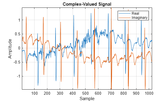
Create a complex-valued signal. Plot the real and imaginary parts of the signal.
load wecg
sig = wecg(1:1024)+1j*wecg(1025:end);
plot([real(sig) imag(sig)])
axis tight
grid on
legend("Real","Imaginary")
title("Complex-Valued Signal")
ylabel("Amplitude")
xlabel("Sample")
Obtain the MODWT of the signal down to level 3 using the db4 wavelet.
lev = 3;
wv = "db4";
wt = modwt(sig,wv,lev);
Create a UI figure window. Add a panel container in the figure.
uif = uifigure(Position=[100 100 720 720]);
p = uipanel(uif,Position=[50 100 600 600], ...
    Title="MRA in Panel Container");
Plot the MRA of the signal on the panel container.
modwtmra(wt,wv,Parent=p)
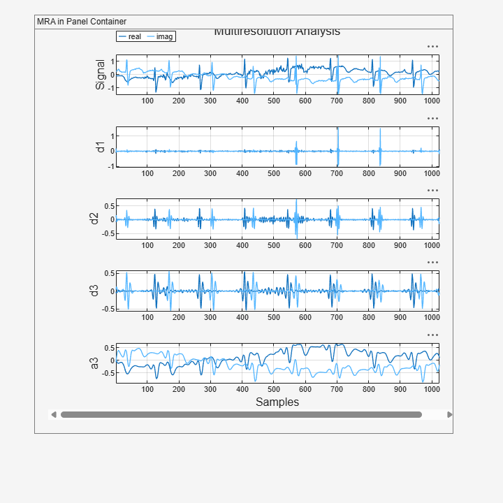
Since R2026a
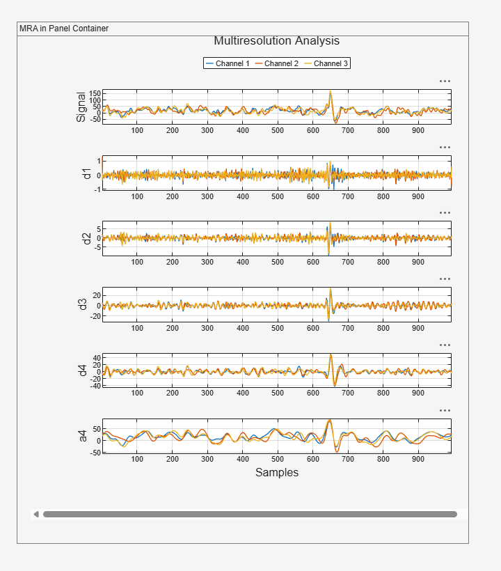
Load the 23 channel EEG data Espiga3 [3]. The channels are arranged column-wise.
load Espiga3Obtain the MODWT of the multisignal down to level four using the db2 wavelet.
wv = "db2";
lev = 4;
wt = modwt(Espiga3,wv,lev);
Create a panel container in a new UI figure.
uif = uifigure(Position=[100 100 720 820]);
p = uipanel(uif,Position=[25 40 650 750], ...
    Title="MRA in Panel Container");
Plot the MRA of the signals in the first, third, and fifth channels on the panel container. In the plot legend, Channel 1, Channel 2, and Channel 3 correspond to the signal in the first, third, and fifth channels, respectively.
modwtmra(wt(:,:,[1 3 5]),wv,Parent=p)
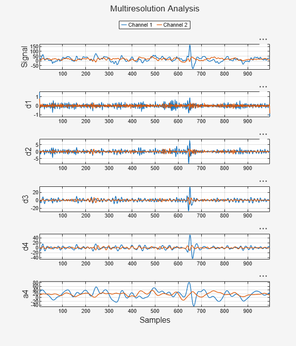
Plot the MRA of the signals in the seventh and tenth channels in a new figure.
figure(Position=[100 100 600 700])
modwtmra(wt(:,:,[7 10]),wv)
Input Arguments
Output Arguments
References
[1] Percival, Donald B., and Andrew T. Walden. Wavelet Methods for Time Series Analysis. Cambridge Series in Statistical and Probabilistic Mathematics. Cambridge ; New York: Cambridge University Press, 2000.
[2] Whitcher, Brandon, Peter Guttorp, and Donald B. Percival. “Wavelet Analysis of Covariance with Application to Atmospheric Time Series.” Journal of Geophysical Research: Atmospheres 105, no. D11 (June 16, 2000): 14941–62. https://doi.org/10.1029/2000JD900110.
[3] Mesa, Hector. “Adapted Wavelets for Pattern Detection.” In Progress in Pattern Recognition, Image Analysis and Applications, edited by Alberto Sanfeliu and Manuel Lazo Cortés, 3773:933–44. Berlin, Heidelberg: Springer Berlin Heidelberg, 2005. https://doi.org/10.1007/11578079_96.