fitlda
Fit latent Dirichlet allocation (LDA) model
Description
A latent Dirichlet allocation (LDA) model is a topic model which discovers underlying topics in a collection of documents and infers word probabilities in topics. If the model was fit using a bag-of-n-grams model, then the software treats the n-grams as individual words.
mdl = fitlda(___,Name,Value)
Examples
To reproduce the results in this example, set rng to 'default'.
rng('default')Load the example data. The file sonnetsPreprocessed.txt contains preprocessed versions of Shakespeare's sonnets. The file contains one sonnet per line, with words separated by a space. Extract the text from sonnetsPreprocessed.txt, split the text into documents at newline characters, and then tokenize the documents.
filename = "sonnetsPreprocessed.txt";
str = extractFileText(filename);
textData = split(str,newline);
documents = tokenizedDocument(textData);
Create a bag-of-words model using bagOfWords.
bag = bagOfWords(documents)
bag =
  bagOfWords with properties:

          Counts: [154×3092 double]
      Vocabulary: ["fairest"    "creatures"    "desire"    "increase"    "thereby"    "beautys"    "rose"    "might"    "never"    "die"    "riper"    "time"    "decease"    "tender"    "heir"    "bear"    "memory"    "thou"    "contracted"    …    ]
        NumWords: 3092
    NumDocuments: 154
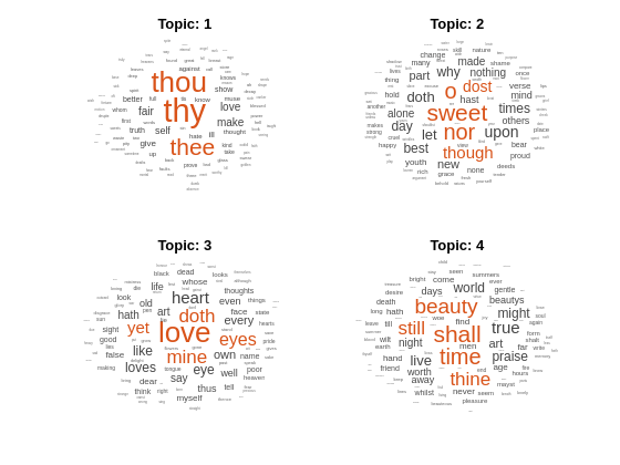
Fit an LDA model with four topics.
numTopics = 4;
mdl = fitlda(bag,numTopics)
Initial topic assignments sampled in 0.263378 seconds.
=====================================================================================
| Iteration  |  Time per  |  Relative  |  Training  |     Topic     |     Topic     |
|            | iteration  | change in  | perplexity | concentration | concentration |
|            | (seconds)  |   log(L)   |            |               |   iterations  |
=====================================================================================
|          0 |       0.17 |            |  1.215e+03 |         1.000 |             0 |
|          1 |       0.02 | 1.0482e-02 |  1.128e+03 |         1.000 |             0 |
|          2 |       0.02 | 1.7190e-03 |  1.115e+03 |         1.000 |             0 |
|          3 |       0.01 | 4.3796e-04 |  1.118e+03 |         1.000 |             0 |
|          4 |       0.01 | 9.4193e-04 |  1.111e+03 |         1.000 |             0 |
|          5 |       0.01 | 3.7079e-04 |  1.108e+03 |         1.000 |             0 |
|          6 |       0.01 | 9.5777e-05 |  1.107e+03 |         1.000 |             0 |
=====================================================================================
mdl =
  ldaModel with properties:

                     NumTopics: 4
             WordConcentration: 1
            TopicConcentration: 1
      CorpusTopicProbabilities: [0.2500 0.2500 0.2500 0.2500]
    DocumentTopicProbabilities: [154×4 double]
        TopicWordProbabilities: [3092×4 double]
                    Vocabulary: ["fairest"    "creatures"    "desire"    "increase"    "thereby"    "beautys"    "rose"    "might"    "never"    "die"    "riper"    "time"    "decease"    "tender"    "heir"    "bear"    "memory"    "thou"    …    ]
                    TopicOrder: 'initial-fit-probability'
                       FitInfo: [1×1 struct]
Visualize the topics using word clouds.
figure
for topicIdx = 1:4
    subplot(2,2,topicIdx)
    wordcloud(mdl,topicIdx);
    title("Topic: " + topicIdx)
end
Fit an LDA model to a collection of documents represented by a word count matrix.
To reproduce the results of this example, set rng to 'default'.
rng('default')Load the example data. sonnetsCounts.mat contains a matrix of word counts and a corresponding vocabulary of preprocessed versions of Shakespeare's sonnets. The value counts(i,j) corresponds to the number of times the jth word of the vocabulary appears in the ith document.
load sonnetsCounts.mat
size(counts)
ans = 1×2
154 3092
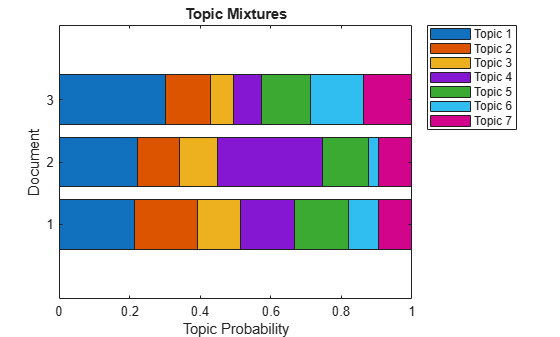
Fit an LDA model with 7 topics. To suppress the verbose output, set 'Verbose' to 0.
numTopics = 7;
mdl = fitlda(counts,numTopics,'Verbose',0);
Visualize multiple topic mixtures using stacked bar charts. Visualize the topic mixtures of the first three input documents.
topicMixtures = transform(mdl,counts(1:3,:));
figure
barh(topicMixtures,'stacked')
xlim([0 1])
title("Topic Mixtures")
xlabel("Topic Probability")
ylabel("Document")
legend("Topic "+ string(1:numTopics),'Location','northeastoutside')
To reproduce the results in this example, set rng to 'default'.
rng('default')Load the example data. The file sonnetsPreprocessed.txt contains preprocessed versions of Shakespeare's sonnets. The file contains one sonnet per line, with words separated by a space. Extract the text from sonnetsPreprocessed.txt, split the text into documents at newline characters, and then tokenize the documents.
filename = "sonnetsPreprocessed.txt";
str = extractFileText(filename);
textData = split(str,newline);
documents = tokenizedDocument(textData);
Create a bag-of-words model using bagOfWords.
bag = bagOfWords(documents)
bag =
  bagOfWords with properties:

          Counts: [154×3092 double]
      Vocabulary: ["fairest"    "creatures"    "desire"    "increase"    "thereby"    "beautys"    "rose"    "might"    "never"    "die"    "riper"    "time"    "decease"    "tender"    "heir"    "bear"    "memory"    "thou"    "contracted"    …    ]
        NumWords: 3092
    NumDocuments: 154
Fit an LDA model with 20 topics.
numTopics = 20;
mdl = fitlda(bag,numTopics)
Initial topic assignments sampled in 0.513255 seconds.
=====================================================================================
| Iteration  |  Time per  |  Relative  |  Training  |     Topic     |     Topic     |
|            | iteration  | change in  | perplexity | concentration | concentration |
|            | (seconds)  |   log(L)   |            |               |   iterations  |
=====================================================================================
|          0 |       0.04 |            |  1.159e+03 |         5.000 |             0 |
|          1 |       0.05 | 5.4884e-02 |  8.028e+02 |         5.000 |             0 |
|          2 |       0.04 | 4.7400e-03 |  7.778e+02 |         5.000 |             0 |
|          3 |       0.04 | 3.4597e-03 |  7.602e+02 |         5.000 |             0 |
|          4 |       0.03 | 3.4662e-03 |  7.430e+02 |         5.000 |             0 |
|          5 |       0.03 | 2.9259e-03 |  7.288e+02 |         5.000 |             0 |
|          6 |       0.03 | 6.4180e-05 |  7.291e+02 |         5.000 |             0 |
=====================================================================================
mdl =
  ldaModel with properties:

                     NumTopics: 20
             WordConcentration: 1
            TopicConcentration: 5
      CorpusTopicProbabilities: [0.0500 0.0500 0.0500 0.0500 0.0500 0.0500 0.0500 0.0500 0.0500 0.0500 0.0500 0.0500 0.0500 0.0500 0.0500 0.0500 0.0500 0.0500 0.0500 0.0500]
    DocumentTopicProbabilities: [154×20 double]
        TopicWordProbabilities: [3092×20 double]
                    Vocabulary: ["fairest"    "creatures"    "desire"    "increase"    "thereby"    "beautys"    "rose"    "might"    "never"    "die"    "riper"    "time"    "decease"    "tender"    "heir"    "bear"    "memory"    "thou"    …    ]
                    TopicOrder: 'initial-fit-probability'
                       FitInfo: [1×1 struct]
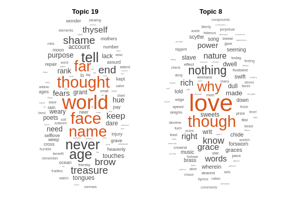
Predict the top topics for an array of new documents.
newDocuments = tokenizedDocument([
    "what's in a name? a rose by any other name would smell as sweet."
    "if music be the food of love, play on."]);
topicIdx = predict(mdl,newDocuments)
topicIdx = 2×1
19
8
Visualize the predicted topics using word clouds.
figure
subplot(1,2,1)
wordcloud(mdl,topicIdx(1));
title("Topic " + topicIdx(1))
subplot(1,2,2)
wordcloud(mdl,topicIdx(2));
title("Topic " + topicIdx(2))
Input Arguments
Name-Value Arguments
Output Arguments
More About
A latent Dirichlet allocation (LDA) model is a document topic model which discovers underlying topics in a collection of documents and infers word probabilities in topics. LDA models a collection of D documents as topic mixtures , over K topics characterized by vectors of word probabilities . The model assumes that the topic mixtures , and the topics follow a Dirichlet distribution with concentration parameters and respectively.
The topic mixtures are probability vectors of length K, where
K is the number of topics. The entry is the probability of topic i appearing in the
dth document. The topic mixtures correspond to the rows of the
DocumentTopicProbabilities property of the ldaModel
object.
The topics are probability vectors of length V, where
V is the number of words in the vocabulary. The entry corresponds to the probability of the vth word of the
vocabulary appearing in the ith topic. The topics correspond to the columns of the TopicWordProbabilities
property of the ldaModel object.
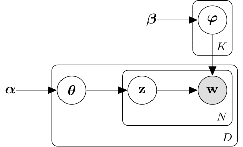
Given the topics and Dirichlet prior on the topic mixtures, LDA assumes the following generative process for a document:
Sample a topic mixture . The random variable is a probability vector of length K, where K is the number of topics.
For each word in the document:
Sample a topic index . The random variable z is an integer from 1 through K, where K is the number of topics.
Sample a word . The random variable w is an integer from 1 through V, where V is the number of words in the vocabulary, and represents the corresponding word in the vocabulary.
Under this generative process, the joint distribution of a document with words , with topic mixture , and with topic indices is given by
where N is the number of words in the document. Summing the joint distribution over z and then integrating over yields the marginal distribution of a document w:
The following diagram illustrates the LDA model as a probabilistic graphical model. Shaded nodes are observed variables, unshaded nodes are latent variables, nodes without outlines are the model parameters. The arrows highlight dependencies between random variables and the plates indicate repeated nodes.
References
[1] Foulds, James, Levi Boyles, Christopher DuBois, Padhraic Smyth, and Max Welling. "Stochastic collapsed variational Bayesian inference for latent Dirichlet allocation." In Proceedings of the 19th ACM SIGKDD international conference on Knowledge discovery and data mining, pp. 446–454. ACM, 2013.
[2] Hoffman, Matthew D., David M. Blei, Chong Wang, and John Paisley. "Stochastic variational inference." The Journal of Machine Learning Research 14, no. 1 (2013): 1303–1347.
[3] Griffiths, Thomas L., and Mark Steyvers. "Finding scientific topics." Proceedings of the National academy of Sciences 101, no. suppl 1 (2004): 5228–5235.
[4] Asuncion, Arthur, Max Welling, Padhraic Smyth, and Yee Whye Teh. "On smoothing and inference for topic models." In Proceedings of the Twenty-Fifth Conference on Uncertainty in Artificial Intelligence, pp. 27–34. AUAI Press, 2009.
[5] Teh, Yee W., David Newman, and Max Welling. "A collapsed variational Bayesian inference algorithm for latent Dirichlet allocation." In Advances in neural information processing systems, pp. 1353–1360. 2007.