Train Linear Regression Model
Statistics and Machine Learning Toolbox™ provides several features for training a linear regression model.
For greater accuracy on low-dimensional through medium-dimensional data sets, use
fitlm. After fitting the model, you can use the object functions to improve, evaluate, and visualize the fitted model. To regularize a regression, uselassoorridge.For reduced computation time on high-dimensional data sets, use
fitrlinear. This function offers useful options for cross-validation, regularization, and hyperparameter optimization.
This example shows the typical workflow for linear regression analysis using fitlm. The workflow includes preparing a data set, fitting a linear regression model, evaluating and improving the fitted model, and predicting response values for new predictor data. The example also describes how to fit and evaluate a linear regression model for tall arrays.
Prepare Data
Load the sample data set NYCHousing2015.
load NYCHousing2015The data set includes 10 variables with information on the sales of properties in New York City in 2015. This example uses some of these variables to analyze the sale prices.
Instead of loading the sample data set NYCHousing2015, you can download the data from the NYC Open Data website and import the data as follows.
folder = 'Annualized_Rolling_Sales_Update';
ds = spreadsheetDatastore(folder,"TextType","string","NumHeaderLines",4);
ds.Files = ds.Files(contains(ds.Files,"2015"));
ds.SelectedVariableNames = ["BOROUGH","NEIGHBORHOOD","BUILDINGCLASSCATEGORY","RESIDENTIALUNITS", ...
    "COMMERCIALUNITS","LANDSQUAREFEET","GROSSSQUAREFEET","YEARBUILT","SALEPRICE","SALEDATE"];
NYCHousing2015 = readall(ds);
Preprocess the data set to choose the predictor variables of interest. First, change the variable names to lowercase for readability.
NYCHousing2015.Properties.VariableNames = lower(NYCHousing2015.Properties.VariableNames);
Next, convert the saledate variable, specified as a datetime array, into two numeric columns MM (month) and DD (day), and remove the saledate variable. Ignore the year values because all samples are for the year 2015.
[~,NYCHousing2015.MM,NYCHousing2015.DD] = ymd(NYCHousing2015.saledate);
NYCHousing2015.saledate = [];
The numeric values in the borough variable indicate the names of the boroughs. Change the variable to a categorical variable using the names.
NYCHousing2015.borough = categorical(NYCHousing2015.borough,1:5, ...
    ["Manhattan","Bronx","Brooklyn","Queens","Staten Island"]);
The neighborhood variable has 254 categories. Remove this variable for simplicity.
NYCHousing2015.neighborhood = [];
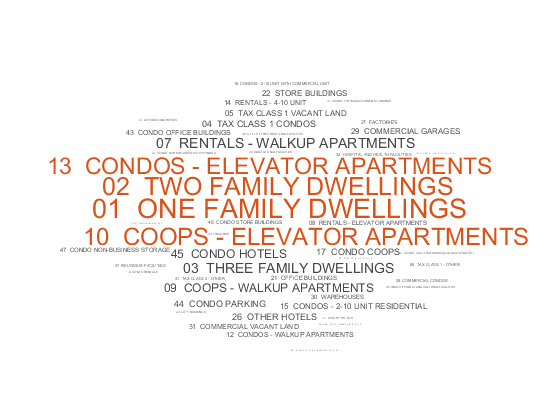
Convert the buildingclasscategory variable to a categorical variable, and explore the variable by using the wordcloud function.
NYCHousing2015.buildingclasscategory = categorical(NYCHousing2015.buildingclasscategory);
wordcloud(NYCHousing2015.buildingclasscategory);
Assume that you are interested only in one-, two-, and three-family dwellings. Find the sample indices for these dwellings and delete the other samples. Then, change the data type of the buildingclasscategory variable to double.
idx = ismember(string(NYCHousing2015.buildingclasscategory), ...
    ["01  ONE FAMILY DWELLINGS","02  TWO FAMILY DWELLINGS","03  THREE FAMILY DWELLINGS"]);
NYCHousing2015 = NYCHousing2015(idx,:);
NYCHousing2015.buildingclasscategory = renamecats(NYCHousing2015.buildingclasscategory, ...
    ["01  ONE FAMILY DWELLINGS","02  TWO FAMILY DWELLINGS","03  THREE FAMILY DWELLINGS"], ...
    ["1","2","3"]);
NYCHousing2015.buildingclasscategory = double(NYCHousing2015.buildingclasscategory);
The buildingclasscategory variable now indicates the number of families in one dwelling.
Explore the response variable saleprice using the summary function.
s = summary(NYCHousing2015);
s.saleprice
ans = struct with fields:
           Size: [37881 1]
           Type: 'double'
    Description: ''
          Units: ''
     Continuity: []
            Min: 0
         Median: 352000
            Max: 37000000
     NumMissing: 0
Assume that a saleprice less than or equal to $1000 indicates ownership transfer without a cash consideration. Remove the samples that have this saleprice.
idx0 = NYCHousing2015.saleprice <= 1000;
NYCHousing2015(idx0,:) = [];
Create a histogram of the saleprice variable.
histogram(NYCHousing2015.saleprice)
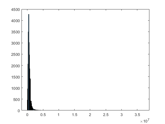
The maximum value of saleprice is , but most values are smaller than . You can identify the outliers of saleprice by using the isoutlier function.
idx = isoutlier(NYCHousing2015.saleprice);
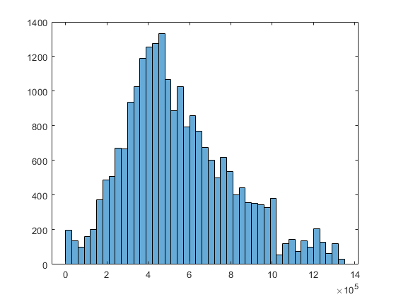
Remove the identified outliers and create the histogram again.
NYCHousing2015(idx,:) = [];
histogram(NYCHousing2015.saleprice)
Partition the data set into a training set and test set by using cvpartition.
rng('default') % For reproducibility
c = cvpartition(height(NYCHousing2015),"holdout",0.3);
trainData = NYCHousing2015(training(c),:);
testData = NYCHousing2015(test(c),:);
Train Model
Fit a linear regression model by using the fitlm function.
mdl = fitlm(trainData,"PredictorVars",["borough","grosssquarefeet", ...
    "landsquarefeet","buildingclasscategory","yearbuilt","MM","DD"], ...
    "ResponseVar","saleprice")
mdl =
Linear regression model:
    saleprice ~ 1 + borough + buildingclasscategory + landsquarefeet + grosssquarefeet + yearbuilt + MM + DD

Estimated Coefficients:
                              Estimate          SE         tStat        pValue
                             ___________    __________    ________    ___________

    (Intercept)               2.0345e+05    1.0308e+05      1.9736       0.048441
    borough_Bronx            -3.0165e+05         56676     -5.3224     1.0378e-07
    borough_Brooklyn              -41160         56490    -0.72862        0.46624
    borough_Queens                -91136         56537      -1.612        0.10699
    borough_Staten Island    -2.2199e+05         56726     -3.9134     9.1385e-05
    buildingclasscategory         3165.7        3510.3     0.90185        0.36715
    landsquarefeet                13.149       0.84534      15.555      3.714e-54
    grosssquarefeet               112.34        2.9494       38.09    8.0393e-304
    yearbuilt                     100.07        45.464       2.201        0.02775
    MM                            3850.5        543.79      7.0808     1.4936e-12
    DD                           -367.19        207.56     -1.7691       0.076896


Number of observations: 15848, Error degrees of freedom: 15837
Root Mean Squared Error: 2.32e+05
R-squared: 0.235,  Adjusted R-Squared: 0.235
F-statistic vs. constant model: 487, p-value = 0
mdl is a LinearModel object. The model display includes the model formula, estimated coefficients, and summary statistics.
borough is a categorical variable that has five categories: Manhattan, Bronx, Brooklyn, Queens, and Staten Island. The fitted model mdl has four indicator variables. The fitlm function uses the first category Manhattan as a reference level, so the model does not include the indicator variable for the reference level. fitlm fixes the coefficient of the indicator variable for the reference level as zero. The coefficient values of the four indicator variables are relative to Manhattan. For more details on how the function treats a categorical predictor, see Algorithms of fitlm.
To learn how to interpret the values in the model display, see Interpret Linear Regression Results.
You can use the properties of a LinearModel object to investigate a fitted linear regression model. The object properties include information about coefficient estimates, summary statistics, fitting method, and input data. For example, you can find the R-squared and adjusted R-squared values in the Rsquared property. You can access the property values through the Workspace browser or using dot notation.
mdl.Rsquared
ans = struct with fields:
    Ordinary: 0.2352
    Adjusted: 0.2348
The model display also shows these values. The R-squared value indicates that the model explains approximately 24% of the variability in the response variable. See Properties of a LinearModel object for details about other properties.
Evaluate Model
The model display shows the p-value of each coefficient. The p-values indicate which variables are significant to the model. For the categorical predictor borough, the model uses four indicator variables and displays four p-values. To examine the categorical variable as a group of indicator variables, use the object function anova. This function returns analysis of variance (ANOVA) statistics of the model.
anova(mdl)
ans=8×5 table
                               SumSq        DF        MeanSq         F         pValue
                             __________    _____    __________    _______    ___________

    borough                   1.123e+14        4    2.8076e+13     520.96              0
    buildingclasscategory    4.3833e+10        1    4.3833e+10    0.81334        0.36715
    landsquarefeet           1.3039e+13        1    1.3039e+13     241.95      3.714e-54
    grosssquarefeet          7.8189e+13        1    7.8189e+13     1450.8    8.0393e-304
    yearbuilt                2.6108e+11        1    2.6108e+11     4.8444        0.02775
    MM                       2.7021e+12        1    2.7021e+12     50.138     1.4936e-12
    DD                       1.6867e+11        1    1.6867e+11     3.1297       0.076896
    Error                     8.535e+14    15837    5.3893e+10
The p-values for the indicator variables borough_Brooklyn and borough_Queens are large, but the p-value of the borough variable as a group of four indicator variables is almost zero, which indicates that the borough variable is statistically significant.
The p-values of buildingclasscategory and DD are larger than 0.05, which indicates that these variables are not significant at the 5% significance level. Therefore, you can consider removing these variables.
You can also use coeffCI, coeefTest, and dwTest to further evaluate the fitted model.
Visualize Model and Summary Statistics
A LinearModel object provides multiple plotting functions.
When creating a model, use
plotAddedto understand the effect of adding or removing a predictor variable.When verifying a model, use
plotDiagnosticsto find questionable data and to understand the effect of each observation. Also, useplotResidualsto analyze the residuals of the model.After fitting a model, use
plotAdjustedResponse,plotPartialDependence, andplotEffectsto understand the effect of a particular predictor. UseplotInteractionto examine the interaction effect between two predictors. Also, useplotSliceto plot slices through the prediction surface.
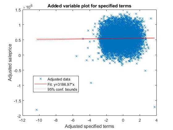
In addition, plot creates an added variable plot for the whole model, except the intercept term, if mdl includes multiple predictor variables.
plot(mdl)
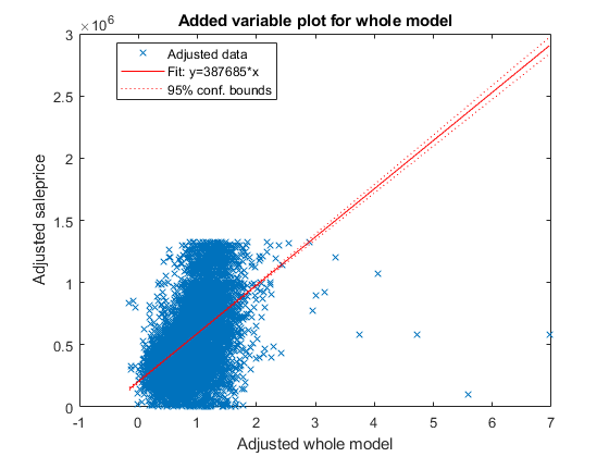
This plot is equivalent to plotAdded(mdl). The fitted line represents how the model, as a group of variables, can explain the response variable. The slope of the fitted line is not close to zero, and the confidence bound does not include a horizontal line, indicating that the model fits better than a degenerate model consisting of only a constant term. The test statistic value shown in the model display (F-statistic vs. constant model) also indicates that the model fits better than the degenerate model.
Create an added variable plot for the insignificant variables buildingclasscategory and DD. The p-values of these variables are larger than 0.05. First, find the indices of these coefficients in mdl.CoefficientNames.
mdl.CoefficientNames
ans = 1×11 cell
    {'(Intercept)'}    {'borough_Bronx'}    {'borough_Brooklyn'}    {'borough_Queens'}    {'borough_Staten Island'}    {'buildingclasscategory'}    {'landsquarefeet'}    {'grosssquarefeet'}    {'yearbuilt'}    {'MM'}    {'DD'}
buildingclasscategory and DD are the 6th and 11th coefficients, respectively. Create an added plot for these two variables.
plotAdded(mdl,[6,11])
The slope of the fitted line is close to zero, indicating that the information from the two variables does not explain the part of the response values not explained by the other predictors. For more details about an added variable plot, see Added Variable Plot.
Create a histogram of the model residuals. plotResiduals plots a histogram of the raw residuals using probability density function scaling.
plotResiduals(mdl)
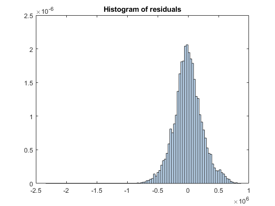
The histogram shows that a few residuals are smaller than . Identify these outliers.
find(mdl.Residuals.Raw < -1*10^6)
ans = 4×1

        1327
        4136
        4997
       13894
Alternatively, you can find the outliers by using isoutlier. Specify the 'grubbs' option to apply Grubbs' test. This option is suitable for a normally distributed data set.
find(isoutlier(mdl.Residuals.Raw,'grubbs'))ans = 3×1
1327
4136
4997
The isoutlier function does not identify residual 13894 as an outlier. This residual is close to –110. Display the residual value.
mdl.Residuals.Raw(13894)
ans = -1.0720e+06
You can exclude outliers when fitting a linear regression model by using the Exclude name-value pair argument. In this case, the example adjusts the fitted model and checks whether the improved model can also explain the outliers.
Adjust Model
Remove the DD and buildingclasscategory variables using removeTerms.
newMdl1 = removeTerms(mdl,"DD + buildingclasscategory")newMdl1 =
Linear regression model:
saleprice ~ 1 + borough + landsquarefeet + grosssquarefeet + yearbuilt + MM
Estimated Coefficients:
Estimate SE tStat pValue
___________ __________ ________ __________
(Intercept) 2.0529e+05 1.0274e+05 1.9981 0.045726
borough_Bronx -3.0038e+05 56675 -5.3 1.1739e-07
borough_Brooklyn -39704 56488 -0.70286 0.48215
borough_Queens -90231 56537 -1.596 0.11052
borough_Staten Island -2.2149e+05 56720 -3.9049 9.4652e-05
landsquarefeet 13.04 0.83912 15.54 4.6278e-54
grosssquarefeet 113.85 2.5078 45.396 0
yearbuilt 96.649 45.395 2.1291 0.033265
MM 3875.6 543.49 7.131 1.0396e-12
Number of observations: 15848, Error degrees of freedom: 15839
Root Mean Squared Error: 2.32e+05
R-squared: 0.235, Adjusted R-Squared: 0.235
F-statistic vs. constant model: 608, p-value = 0
Because the two variables are not significant in explaining the response variable, the R-squared and adjusted R-squared values of newMdl1 are close to the values of mdl.
Improve the model by adding or removing variables using step. The default upper bound of the model is a model containing an intercept term, the linear term for each predictor, and all products of pairs of distinct predictors (no squared terms), and the default lower bound is a model containing an intercept term. Specify the maximum number of steps to take as 30. The function stops when no single step improves the model.
newMdl2 = step(newMdl1,'NSteps',30)1. Adding borough:grosssquarefeet, FStat = 58.7413, pValue = 2.63078e-49 2. Adding borough:yearbuilt, FStat = 31.5067, pValue = 3.50645e-26 3. Adding borough:landsquarefeet, FStat = 29.5473, pValue = 1.60885e-24 4. Adding grosssquarefeet:yearbuilt, FStat = 69.312, pValue = 9.08599e-17 5. Adding landsquarefeet:grosssquarefeet, FStat = 33.2929, pValue = 8.07535e-09 6. Adding landsquarefeet:yearbuilt, FStat = 45.2756, pValue = 1.7704e-11 7. Adding yearbuilt:MM, FStat = 18.0785, pValue = 2.13196e-05 8. Adding residentialunits, FStat = 16.0491, pValue = 6.20026e-05 9. Adding residentialunits:landsquarefeet, FStat = 160.2601, pValue = 1.49309e-36 10. Adding residentialunits:grosssquarefeet, FStat = 27.351, pValue = 1.71835e-07 11. Adding commercialunits, FStat = 14.1503, pValue = 0.000169381 12. Adding commercialunits:grosssquarefeet, FStat = 25.6942, pValue = 4.04549e-07 13. Adding borough:commercialunits, FStat = 6.1327, pValue = 6.3015e-05 14. Adding buildingclasscategory, FStat = 11.1412, pValue = 0.00084624 15. Adding buildingclasscategory:landsquarefeet, FStat = 66.9205, pValue = 3.04003e-16 16. Adding buildingclasscategory:yearbuilt, FStat = 15.0776, pValue = 0.0001036 17. Adding buildingclasscategory:grosssquarefeet, FStat = 18.3304, pValue = 1.86812e-05 18. Adding residentialunits:yearbuilt, FStat = 15.0732, pValue = 0.00010384 19. Adding buildingclasscategory:residentialunits, FStat = 13.5644, pValue = 0.00023129 20. Adding borough:buildingclasscategory, FStat = 2.8214, pValue = 0.023567 21. Adding landsquarefeet:MM, FStat = 4.9185, pValue = 0.026585 22. Removing grosssquarefeet:yearbuilt, FStat = 1.6052, pValue = 0.20519
newMdl2 =
Linear regression model:
    saleprice ~ 1 + borough*buildingclasscategory + borough*commercialunits + borough*landsquarefeet + borough*grosssquarefeet + borough*yearbuilt + buildingclasscategory*residentialunits + buildingclasscategory*landsquarefeet + buildingclasscategory*grosssquarefeet + buildingclasscategory*yearbuilt + residentialunits*landsquarefeet + residentialunits*grosssquarefeet + residentialunits*yearbuilt + commercialunits*grosssquarefeet + landsquarefeet*grosssquarefeet + landsquarefeet*yearbuilt + landsquarefeet*MM + yearbuilt*MM

Estimated Coefficients:
                                                    Estimate          SE         tStat        pValue
                                                   ___________    __________    ________    __________

    (Intercept)                                     2.2152e+07     1.318e+07      1.6808      0.092825
    borough_Bronx                                  -2.3263e+07    1.3176e+07     -1.7656      0.077486
    borough_Brooklyn                               -1.8935e+07    1.3174e+07     -1.4373       0.15064
    borough_Queens                                 -2.1757e+07    1.3173e+07     -1.6516      0.098636
    borough_Staten Island                          -2.3471e+07    1.3177e+07     -1.7813      0.074891
    buildingclasscategory                          -7.2403e+05    1.9374e+05      -3.737    0.00018685
    residentialunits                                6.1912e+05    1.2399e+05      4.9932     6.003e-07
    commercialunits                                 4.2016e+05    1.2815e+05      3.2786     0.0010456
    landsquarefeet                                     -390.54        96.349     -4.0535    5.0709e-05
    grosssquarefeet                                     189.33        83.723      2.2614      0.023748
    yearbuilt                                           -11556        6958.7     -1.6606      0.096805
    MM                                                   95189         31787      2.9946     0.0027521
    borough_Bronx:buildingclasscategory            -1.1972e+05    1.0481e+05     -1.1422       0.25338
    borough_Brooklyn:buildingclasscategory         -1.4154e+05    1.0448e+05     -1.3548       0.17551
    borough_Queens:buildingclasscategory           -1.1597e+05    1.0454e+05     -1.1093        0.2673
    borough_Staten Island:buildingclasscategory    -1.1851e+05    1.0513e+05     -1.1273       0.25964
    borough_Bronx:commercialunits                  -2.7488e+05    1.3267e+05     -2.0719      0.038293
    borough_Brooklyn:commercialunits               -3.8228e+05    1.2835e+05     -2.9784     0.0029015
    borough_Queens:commercialunits                 -3.9818e+05    1.2884e+05     -3.0906     0.0020008
    borough_Staten Island:commercialunits          -4.9381e+05     1.353e+05     -3.6496    0.00026348
    borough_Bronx:landsquarefeet                        121.81        77.442       1.573       0.11574
    borough_Brooklyn:landsquarefeet                     113.09        77.413      1.4609       0.14405
    borough_Queens:landsquarefeet                       99.894        77.374      1.2911        0.1967
    borough_Staten Island:landsquarefeet                84.508        77.376      1.0922       0.27477
    borough_Bronx:grosssquarefeet                      -55.417        83.412    -0.66437       0.50646
    borough_Brooklyn:grosssquarefeet                    6.4033        83.031    0.077119       0.93853
    borough_Queens:grosssquarefeet                       38.28        83.144     0.46041       0.64523
    borough_Staten Island:grosssquarefeet               12.539        83.459     0.15024       0.88058
    borough_Bronx:yearbuilt                              12121        6956.8      1.7422      0.081485
    borough_Brooklyn:yearbuilt                          9986.5        6955.8      1.4357        0.1511
    borough_Queens:yearbuilt                             11382        6955.3      1.6364       0.10177
    borough_Staten Island:yearbuilt                      12237        6957.1      1.7589      0.078613
    buildingclasscategory:residentialunits               21392          5465      3.9143    9.1041e-05
    buildingclasscategory:landsquarefeet               -13.099        2.0014      -6.545    6.1342e-11
    buildingclasscategory:grosssquarefeet              -30.087        5.2786     -5.6998    1.2209e-08
    buildingclasscategory:yearbuilt                     462.31        85.912      5.3813    7.5021e-08
    residentialunits:landsquarefeet                    -1.0826       0.13896     -7.7911    7.0554e-15
    residentialunits:grosssquarefeet                   -5.1192        1.7923     -2.8563     0.0042917
    residentialunits:yearbuilt                         -326.69        63.556     -5.1403    2.7762e-07
    commercialunits:grosssquarefeet                    -29.839        5.0231     -5.9403    2.9045e-09
    landsquarefeet:grosssquarefeet                  -0.0055199     0.0010364     -5.3262    1.0165e-07
    landsquarefeet:yearbuilt                            0.1766      0.030902      5.7151    1.1164e-08
    landsquarefeet:MM                                   0.6595       0.30229      2.1817      0.029145
    yearbuilt:MM                                       -47.944        16.392     -2.9248     0.0034512


Number of observations: 15848, Error degrees of freedom: 15804
Root Mean Squared Error: 2.25e+05
R-squared: 0.285,  Adjusted R-Squared: 0.283
F-statistic vs. constant model: 146, p-value = 0
The R-squared and adjusted R-squared values of newMdl2 are larger than the values of newMdl1.
Create a histogram of the model residuals by using plotResiduals.
plotResiduals(newMdl2)
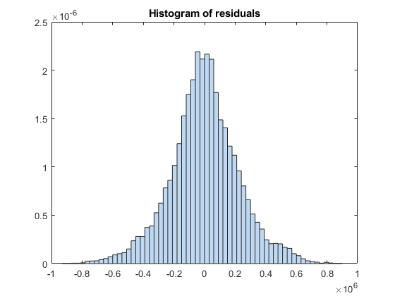
The residual histogram of newMdl2 is symmetric, without outliers.
You can also use addTerms to add specific terms. Alternatively, you can use stepwiselm to specify terms in a starting model and continue improving the model by using stepwise regression.
Predict Responses to New Data
Predict responses to the test data set testData by using the fitted model newMdl2 and the object function predict to
ypred = predict(newMdl2,testData);
Plot the residual histogram of the test data set.
errs = ypred - testData.saleprice;
histogram(errs)
title("Histogram of residuals - test data")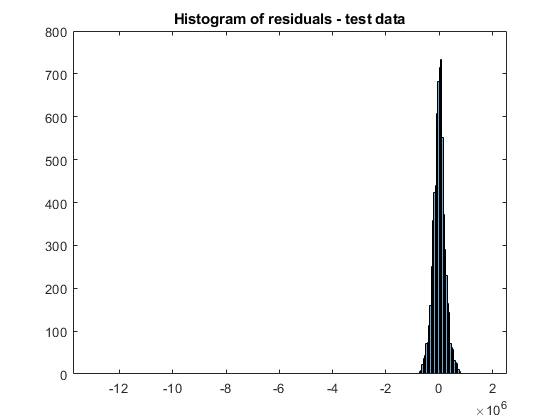
The residual values have a few outliers.
errs(isoutlier(errs,'grubbs'))ans = 6×1
107 ×
0.1788
-0.4688
-1.2981
0.1019
0.1122
0.1331
Analyze Using Tall Arrays
The fitlm function supports tall arrays for out-of-memory data, with some limitations. For tall data, fitlm returns a CompactLinearModel object that contains most of the same properties as a LinearModel object. The main difference is that the compact object is sensitive to memory requirements. The compact object does not have properties that include the data, or that include an array of the same size as the data. Therefore, some LinearModel object functions that require data do not work with a compact model. See Object Functions for the list of supported object functions. Also, see Tall Arrays for the usage notes and limitations of fitlm for tall arrays.
When you perform calculations on tall arrays, MATLAB® uses either a parallel pool (default if you have Parallel Computing Toolbox™) or the local MATLAB session. If you want to run the example using the local MATLAB session when you have Parallel Computing Toolbox, you can change the global execution environment by using the mapreducer function.
Assume that all the data in the datastore ds does not fit in memory. You can use tall instead of readall to read ds.
NYCHousing2015 = tall(ds);
For this example, convert the in-memory table NYCHousing2015 to a tall table by using the tall function.
NYCHousing2015_t = tall(NYCHousing2015);
Starting parallel pool (parpool) using the 'local' profile ...
Connected to the parallel pool (number of workers: 6).
Partition the data set into a training set and test set. When you use cvpartition with tall arrays, the function partitions the data set based on the variable supplied as the first input argument. For classification problems, you typically use the response variable (a grouping variable) and create a random stratified partition to get even distribution between training and test sets for all groups. For regression problems, this stratification is not adequate, and you can use the 'Stratify' name-value pair argument to turn off the option.
In this example, specify the predictor variable NYCHousing2015_t.borough as the first input argument to make the distribution of boroughs roughly the same across the training and tests sets. For reproducibility, set the seed of the random number generator using tallrng. The results can vary depending on the number of workers and the execution environment for the tall arrays. For details, see Control Where Your Code Runs.
tallrng('default') % For reproducibility
c = cvpartition(NYCHousing2015_t.borough,"holdout",0.3);
trainData_t = NYCHousing2015_t(training(c),:);
testData_t = NYCHousing2015_t(test(c),:);
Because fitlm returns a compact model object for tall arrays, you cannot improve the model using the step function. Instead, you can explore the model parameters by using the object functions and then adjust the model as needed. You can also gather a subset of the data into the workspace, use stepwiselm to iteratively develop the model in memory, and then scale up to use tall arrays. For details, see Model Development of Statistics and Machine Learning with Big Data Using Tall Arrays.
In this example, fit a linear regression model using the model formula of newMdl2.
mdl_t = fitlm(trainData_t,newMdl2.Formula)
Evaluating tall expression using the Parallel Pool 'local':
- Pass 1 of 1: Completed in 7.4 sec
Evaluation completed in 9.2 sec
mdl_t =
Compact linear regression model:
    saleprice ~ 1 + borough*buildingclasscategory + borough*commercialunits + borough*landsquarefeet + borough*grosssquarefeet + borough*yearbuilt + buildingclasscategory*residentialunits + buildingclasscategory*landsquarefeet + buildingclasscategory*grosssquarefeet + buildingclasscategory*yearbuilt + residentialunits*landsquarefeet + residentialunits*grosssquarefeet + residentialunits*yearbuilt + commercialunits*grosssquarefeet + landsquarefeet*grosssquarefeet + landsquarefeet*yearbuilt + landsquarefeet*MM + yearbuilt*MM

Estimated Coefficients:
                                                    Estimate          SE         tStat        pValue
                                                   ___________    __________    ________    __________

    (Intercept)                                    -1.3301e+06    5.1815e+05      -2.567      0.010268
    borough_Brooklyn                                4.2583e+06    4.1808e+05      10.185    2.7392e-24
    borough_Manhattan                               2.2758e+07    1.3448e+07      1.6923      0.090614
    borough_Queens                                  1.1395e+06    4.1868e+05      2.7216     0.0065035
    borough_Staten Island                          -1.1196e+05    4.6677e+05    -0.23986       0.81044
    buildingclasscategory                            -8.08e+05    1.6219e+05     -4.9817    6.3705e-07
    residentialunits                                6.0588e+05    1.2669e+05      4.7822    1.7497e-06
    commercialunits                                      80197         53311      1.5043       0.13252
    landsquarefeet                                     -279.94        53.913     -5.1925    2.1009e-07
    grosssquarefeet                                     170.02        13.996      12.147    8.3837e-34
    yearbuilt                                           683.49        268.34      2.5471      0.010872
    MM                                                   86488         32725      2.6428     0.0082293
    borough_Brooklyn:buildingclasscategory             -9852.4         12048    -0.81773       0.41352
    borough_Manhattan:buildingclasscategory         1.3318e+05    1.3592e+05     0.97988       0.32716
    borough_Queens:buildingclasscategory                 15621         11671      1.3385       0.18076
    borough_Staten Island:buildingclasscategory          15132         14893       1.016       0.30964
    borough_Brooklyn:commercialunits                    -22060         43012    -0.51289       0.60804
    borough_Manhattan:commercialunits               4.8349e+05    2.1757e+05      2.2222      0.026282
    borough_Queens:commercialunits                      -42023         44736    -0.93936       0.34756
    borough_Staten Island:commercialunits          -1.3382e+05         56976     -2.3487      0.018853
    borough_Brooklyn:landsquarefeet                     9.8263        5.2513      1.8712      0.061335
    borough_Manhattan:landsquarefeet                   -78.962        78.445     -1.0066       0.31415
    borough_Queens:landsquarefeet                      -3.0855        3.9087    -0.78939        0.4299
    borough_Staten Island:landsquarefeet               -17.325        3.5831     -4.8351    1.3433e-06
    borough_Brooklyn:grosssquarefeet                    37.689        10.573      3.5646    0.00036548
    borough_Manhattan:grosssquarefeet                   16.107        82.074     0.19625       0.84442
    borough_Queens:grosssquarefeet                      70.381         10.69      6.5837    4.7343e-11
    borough_Staten Island:grosssquarefeet               36.396         12.08      3.0129     0.0025914
    borough_Brooklyn:yearbuilt                         -2110.1        216.32     -9.7546    2.0388e-22
    borough_Manhattan:yearbuilt                         -11884        7023.9      -1.692      0.090667
    borough_Queens:yearbuilt                           -566.44        216.89     -2.6116     0.0090204
    borough_Staten Island:yearbuilt                     53.714        239.89     0.22391       0.82283
    buildingclasscategory:residentialunits               24088          5574      4.3215    1.5595e-05
    buildingclasscategory:landsquarefeet                5.7964        5.8438      0.9919       0.32126
    buildingclasscategory:grosssquarefeet              -47.079        5.2884     -8.9023    6.0556e-19
    buildingclasscategory:yearbuilt                     430.97        83.593      5.1555      2.56e-07
    residentialunits:landsquarefeet                    -21.756        5.6485     -3.8517    0.00011778
    residentialunits:grosssquarefeet                     4.584        1.4586      3.1427     0.0016769
    residentialunits:yearbuilt                         -310.09        65.429     -4.7393    2.1632e-06
    commercialunits:grosssquarefeet                    -27.839        11.463     -2.4286      0.015166
    landsquarefeet:grosssquarefeet                  -0.0068613    0.00094607     -7.2524    4.2832e-13
    landsquarefeet:yearbuilt                           0.17489      0.028195      6.2028    5.6861e-10
    landsquarefeet:MM                                  0.70295        0.2848      2.4682      0.013589
    yearbuilt:MM                                       -43.405        16.871     -2.5728      0.010098


Number of observations: 15849, Error degrees of freedom: 15805
Root Mean Squared Error: 2.26e+05
R-squared: 0.277,  Adjusted R-Squared: 0.275
F-statistic vs. constant model: 141, p-value = 0
mdl_t is a CompactLinearModel object. mdl_t is not exactly the same as newMdl2 because the partitioned training data set obtained from the tall table is not the same as the one from the in-memory data set.
You cannot use the plotResiduals function to create a histogram of the model residuals because mdl_t is a compact object. Instead, compute the residuals directly from the compact object and create the histogram using histogram.
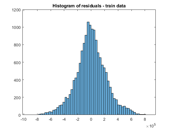
mdl_t_Residual = trainData_t.saleprice - predict(mdl_t,trainData_t);
histogram(mdl_t_Residual)
Evaluating tall expression using the Parallel Pool 'local':
- Pass 1 of 2: Completed in 2.5 sec
- Pass 2 of 2: Completed in 0.63 sec
Evaluation completed in 3.8 sec
title("Histogram of residuals - train data")Predict responses to the test data set testData_t by using predict.
ypred_t = predict(mdl_t,testData_t);
Plot the residual histogram of the test data set.
errs_t = ypred_t - testData_t.saleprice;
histogram(errs_t)
Evaluating tall expression using the Parallel Pool 'local':
- Pass 1 of 2: 0% complete
Evaluation 0% complete
- Pass 1 of 2: 6% complete
Evaluation 3% complete
- Pass 1 of 2: Completed in 0.79 sec
- Pass 2 of 2: Completed in 0.55 sec
Evaluation completed in 2 sec
title("Histogram of residuals - test data")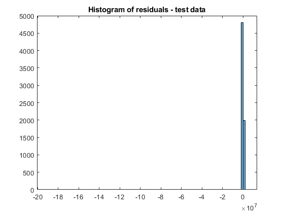
You can further assess the fitted model using the CompactLinearModel object functions. For an example, see Assess and Adjust Model of Statistics and Machine Learning with Big Data Using Tall Arrays.
See Also
isoutlier | fitlm | LinearModel | CompactLinearModel
Topics
- Linear Regression
- Linear Regression Workflow
- Interpret Linear Regression Results
- Linear Regression with Interaction Effects
- Linear Regression with Categorical Covariates
- Examine Quality and Adjust Fitted Model
- Summary of Output and Diagnostic Statistics
- Statistics and Machine Learning with Big Data Using Tall Arrays