Linear Regression Workflow
This example shows how to fit a linear regression model. A typical workflow involves the following: import data, fit a regression, test its quality, modify it to improve the quality, and share it.
Step 1. Import the data into a table.
hospital.xls is an Excel® spreadsheet containing patient names, sex, age, weight, blood pressure, and dates of treatment in an experimental protocol. First read the data into a table.
patients = readtable('hospital.xls','ReadRowNames',true);
Examine the five rows of data.
patients(1:5,:)
ans=5×11 table
                   name         sex     age    wgt    smoke    sys    dia    trial1    trial2    trial3    trial4
               ____________    _____    ___    ___    _____    ___    ___    ______    ______    ______    ______

    YPL-320    {'SMITH'   }    {'m'}    38     176      1      124    93       18       -99       -99       -99
    GLI-532    {'JOHNSON' }    {'m'}    43     163      0      109    77       11        13        22       -99
    PNI-258    {'WILLIAMS'}    {'f'}    38     131      0      125    83      -99       -99       -99       -99
    MIJ-579    {'JONES'   }    {'f'}    40     133      0      117    75        6        12       -99       -99
    XLK-030    {'BROWN'   }    {'f'}    49     119      0      122    80       14        23       -99       -99
The sex and smoke fields seem to have two choices each. So change these fields to categorical.
patients.smoke = categorical(patients.smoke,0:1,{'No','Yes'});
patients.sex = categorical(patients.sex);
Step 2. Create a fitted model.
Your goal is to model the systolic pressure as a function of a patient's age, weight, sex, and smoking status. Create a linear formula for 'sys' as a function of 'age', 'wgt', 'sex', and 'smoke'.
modelspec = 'sys ~ age + wgt + sex + smoke';
mdl = fitlm(patients,modelspec)
mdl =
Linear regression model:
sys ~ 1 + sex + age + wgt + smoke
Estimated Coefficients:
Estimate SE tStat pValue
_________ ________ ________ __________
(Intercept) 118.28 7.6291 15.504 9.1557e-28
sex_m 0.88162 2.9473 0.29913 0.76549
age 0.08602 0.06731 1.278 0.20438
wgt -0.016685 0.055714 -0.29947 0.76524
smoke_Yes 9.884 1.0406 9.498 1.9546e-15
Number of observations: 100, Error degrees of freedom: 95
Root Mean Squared Error: 4.81
R-squared: 0.508, Adjusted R-Squared: 0.487
F-statistic vs. constant model: 24.5, p-value = 5.99e-14
The sex, age, and weight predictors have rather high -values, indicating that some of these predictors might be unnecessary.
Step 3. Locate and remove outliers.
See if there are outliers in the data that should be excluded from the fit. Plot the residuals.
plotResiduals(mdl)
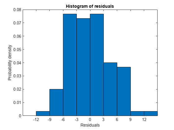
There is one possible outlier, with a value greater than 12. This is probably not truly an outlier. For demonstration, here is how to find and remove it.
Find the outlier.
outlier = mdl.Residuals.Raw > 12;
find(outlier)
ans =
84
Remove the outlier.
mdl = fitlm(patients,modelspec,...
    'Exclude',84);

mdl.ObservationInfo(84,:)
ans=1×4 table
               Weights    Excluded    Missing    Subset
               _______    ________    _______    ______

    WXM-486       1        true        false     false
Observation 84 is no longer in the model.
Step 4. Simplify the model.
Try to obtain a simpler model, one with fewer predictors but the same predictive accuracy. step looks for a better model by adding or removing one term at a time. Allow step take up to 10 steps.
mdl1 = step(mdl,'NSteps',10)1. Removing wgt, FStat = 4.6001e-05, pValue = 0.9946 2. Removing sex, FStat = 0.063241, pValue = 0.80199
mdl1 =
Linear regression model:
    sys ~ 1 + age + smoke

Estimated Coefficients:
                   Estimate       SE       tStat       pValue
                   ________    ________    ______    __________

    (Intercept)     115.11       2.5364    45.383    1.1407e-66
    age            0.10782     0.064844    1.6628       0.09962
    smoke_Yes       10.054      0.97696    10.291    3.5276e-17


Number of observations: 99, Error degrees of freedom: 96
Root Mean Squared Error: 4.61
R-squared: 0.536,  Adjusted R-Squared: 0.526
F-statistic vs. constant model: 55.4, p-value = 1.02e-16
step took two steps. This means it could not improve the model further by adding or subtracting a single term.
Plot the effectiveness of the simpler model on the training data.
plotResiduals(mdl1)
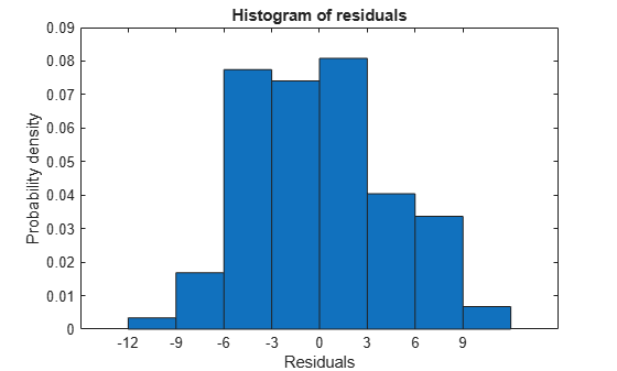
The residuals look about as small as those of the original model.
Step 5. Predict responses to new data.
Suppose you have four new people, aged 25, 30, 40, and 65, and the first and third smoke. Predict their systolic pressure using mdl1.
ages = [25;30;40;65];
smoker = {'Yes';'No';'Yes';'No'};
systolicnew = feval(mdl1,ages,smoker)
systolicnew = 4×1
127.8561
118.3412
129.4734
122.1149
To make predictions, you need only the variables that mdl1 uses.
Step 6. Share the model.
You might want others to be able to use your model for prediction. Access the terms in the linear model.
coefnames = mdl1.CoefficientNames
coefnames = 1×3 cell
    {'(Intercept)'}    {'age'}    {'smoke_Yes'}
View the model formula.
mdl1.Formula
ans =
sys ~ 1 + age + smoke
Access the coefficients of the terms.
coefvals = mdl1.Coefficients(:,1).Estimate
coefvals = 3×1

  115.1066
    0.1078
   10.0540
The model is sys = 115.1066 + 0.1078*age + 10.0540*smoke, where smoke is 1 for a smoker, and 0 otherwise.
See Also
fitlm | LinearModel | feval | step | plotResiduals