impulseest
Nonparametric impulse response estimation
Syntax
Description
sys = impulseest(data)sys, also known as a finite
impulse response (FIR) model, using time-domain or frequency-domain data
data.
data can be in the form of a timetable, a comma-separated pair of numeric matrices, or an iddata object. If
data is a timetable, the software assumes that the last
variable is the single output. You can select specific input and output channels to
use for estimation by specifying the channel names in the
InputName and OutputName name-value
arguments.
The function uses persistence-of-excitation analysis on the input data to select the model order (number of nonzero impulse response coefficients).
Use nonparametric impulse response estimation to analyze input/output data for feedback effects, delays, and significant time constants.
sys = impulseest(___,Name,Value)sys =
impulseest(data,'InputName',["u1","u3"],'OutputName',["y1","y4"]).
You can use this syntax with any of the previous input-argument combinations.
Examples
Estimate a nonparametric impulse response model using data from a hair dryer. The input is the voltage applied to the heater and the output is the heater temperature. Use the first 500 samples for estimation.
Load the data and use the first 500 samples to estimate the model.
load dry2data dry2tt
tte = dry2tt(1:500,:);
sys = impulseest(tte);
tte is a timetable that contains time-domain data. sys, the identified nonparametric impulse response model, is an idtf model.
Analyze the impulse response of the identified model from time 0 to 1.
h = impulseplot(sys,1);
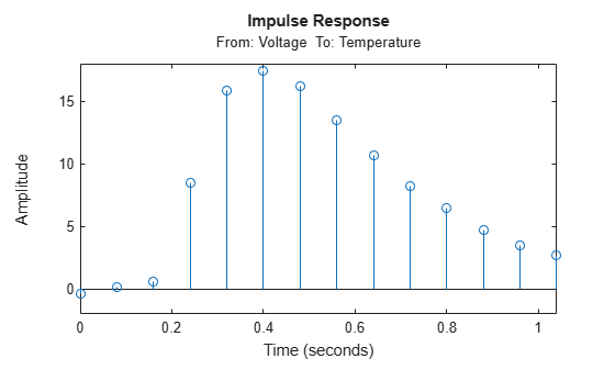
Determine the point at which a significant response to the impulse begins. First, display the region that bounds amplitudes that are not significantly different from zero. To do so, right-click the plot and select Characteristics > Confidence Region. For impulse response plots, by default, this selection displays a confidence region with a width of one standard deviation that is centered at zero, instead of one centered at the response values. You can modify these defaults by right-clicking the plot and selecting Properties > Options.
Alternatively, you can use the showConfidence command.
showConfidence(h);
The first response value that is significantly different than zero occurs at 0.24 seconds, or the third sample. This implies that the transport delay is three samples. To generate a model that imposes the three-sample delay, set the transport delay, which is the third argument, to 3. You must also set the second argument, the order n, to its default value of [] as a placeholder.
sys1 = impulseest(tte,[],3);
h1 = impulseplot(sys1,1);
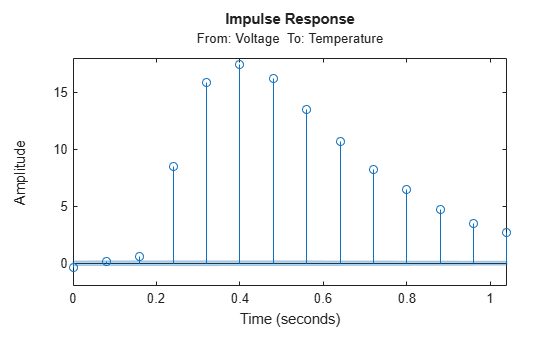
showConfidence(h1);

The response is identically zero until 0.24 seconds.
Load the estimation data.
load sdata3 umat3 ymat3 Ts;
Estimate a 35th-order FIR model.
n = 35;
sys = impulseest(umat3,ymat3,n);
You can confirm the model order of sys by displaying the number of terms.
nsys = size(sys.num)
nsys = 1×2

     1    35
Set n to [] so that the function automatically determines n. Display the model order.
n = [];
sys1 = impulseest(umat3,ymat3,n);
nsys1 = size(sys1.Numerator)
nsys1 = 1×2

     1    70
The model order is 70. The default value for the order is [], so setting the order to [] is equivalent to omitting the specification.
Estimate an impulse response model with a transport delay of 3 samples.
If you know about the presence of delay in the input/output data in advance, use the delay value as a transport delay for impulse response estimation.
Generate data that contains a 3-sample input-to-output lag.
Create a random input signal. Construct an idpoly model that includes three sample delays, which you implement by using three leading zeros in the B polynomial.
u = rand(100,1);
A = [1 .1 .4];
B = [0 0 0 4 -2];
C = [1 1 .1];
sys = idpoly(A,B,C);
Simulate the model response y to the noise signal, using the AddNoise option and a sample time of 1 second. Encapsulate y in an iddata object.
opt = simOptions('AddNoise',true);
y = sim(sys,u,opt);
data = iddata(y,u,1);
Estimate and plot a 20th order model with no transport delay.
n = 20;
model1 = impulseest(data,n);
impulseplot(model1);

The plot shows that the impulse response includes nonzero samples during the 3-second delay period.
Estimate a model with a 3-sample transport delay.
nk = 3;
model2 = impulseest(data,n,nk);
impulseplot(model2)

The first three samples are identically zero.
Obtain regularized estimates of impulse response model using the regularizing kernel estimation option.
Estimate a model using regularization. impulseest performs regularized estimates by default, using the tuned and correlated kernel ('TC').
load iddata3 z3;
sys1 = impulseest(z3);
Estimate a model with no regularization.
opt = impulseestOptions('RegularizationKernel','none');
sys2 = impulseest(z3,opt);
Compare the impulse responses of both models.
h = impulseplot(sys2,sys1,70);
legend('sys2','sys1')
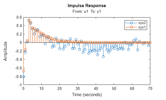
As the plot shows, using regularization makes the response smoother.
Plot the confidence intervals.
showConfidence(h);
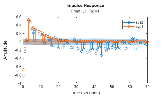
The uncertainty in the computed response is reduced at larger lags for the model using regularization. Regularization decreases variance at the price of some bias. The tuning of the 'TC' regularization is such that the variance error dominates the overall error.
Load the estimation data.
load regularizationExampleData eData;
Recreate the transfer function model that was used for generating the estimation data (true system).
num = [0.02008 0.04017 0.02008];
den = [1 -1.561 0.6414];
Ts = 1;
trueSys = idtf(num,den,Ts);
Obtain a regularized impulse response (FIR) model with an order of 70.
opt = impulseestOptions('RegularizationKernel','DC');
m0 = impulseest(eData,70,opt);
Convert the model into a state-space model and reduce the model order.
m1 = idss(m0);
m1 = balred(m1,15);
Estimate a second state-space model directly from eData by using regularized reduction of an ARX model.
m2 = ssregest(eData,15);
Compare the impulse responses of the true system and the estimated models.
impulse(trueSys,m1,m2,50);
legend('trueSys','m1','m2');
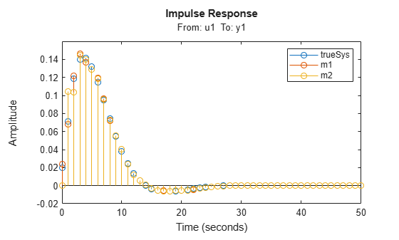
The three model responses are similar.
Use the empirical impulse response to measured data to determine whether the data includes feedback effects. Feedback effects can be present when the impulse response includes statistically significant response values for negative time values.
Compute the noncausal impulse response using a fourth-order prewhitening filter and no regularization, automatic order selection, and negative lag.
load iddata3 z3;
opt = impulseestOptions('pw',4,'RegularizationKernel','none');
sys = impulseest(z3,[],'negative',opt);
sys is a noncausal model containing response values for negative time.
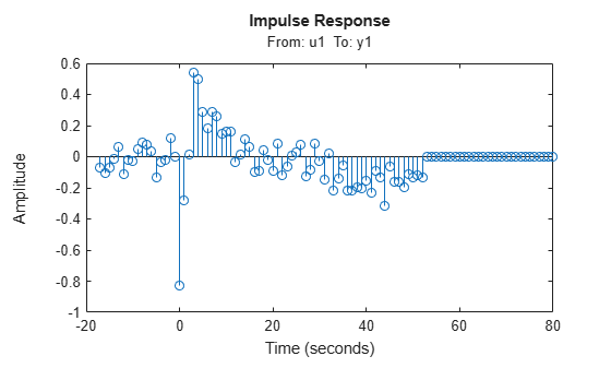
Analyze the impulse response of the identified model.
h = impulseplot(sys);
View the zero-response region at one standard deviation by right-clicking on the plot and selecting Characteristics > Confidence Region. Alternatively, you can use the showConfidence command.
showConfidence(h);
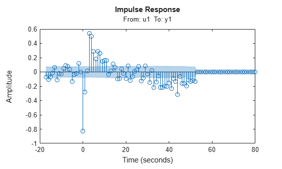
The large response value at t=0 (zero lag) suggests that the data comes from a process containing feedthrough. That is, the input affects the output instantaneously. The large response value can also indicate direct feedback, such as proportional control without some delay so that y(t) partly determines u(t).
Other indications of feedback in the data are the significant response values such as those at -7 seconds and -9 seconds.
Compute an impulse response model for frequency response data.
Load the frequency response data, which contains measured amplitude AMP and phase PHA for the frequency vector W.
load demofr;Create the complex frequency response zfr and encapsulate it in an idfrd object that has a sample time of 0.1 seconds. Plot the data.
zfr = AMP.*exp(1i*PHA*pi/180);
Ts = 0.1;
data = idfrd(zfr,W,Ts);
Estimate an impulse response model from data and plot the response.
sys = impulseest(data);
impulseplot(sys)

Identify parametric and nonparametric models for a data set, and compare their step responses.
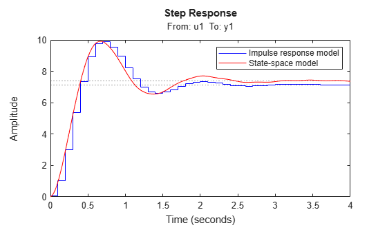
Estimate the impulse response model sys1 (nonparametric) and state-space model sys2 (parametric) using the estimation data set z1.
load iddata1 z1;
sys1 = impulseest(z1);
sys2 = ssest(z1,4);
sys1 is a discrete-time identified transfer function model. sys2 is a continuous-time identified state-space model.
Compare the step responses for sys1 and sys2.
step(sys1,'b',sys2,'r');
legend('Impulse response model','State-space model');
Input Arguments
Name-Value Arguments
Output Arguments
Tips
To view the impulse or step response of
sys, use eitherimpulseplotorstepplot, respectively.A response value that corresponds to a negative time value and that is significantly different from zero in the impulse response of
sysindicates the presence of feedback in the data.To view the region of responses that are not significantly different from zero (the zero-response region) in a plot, right-click on the plot and select Characteristics > Confidence Region. A patch depicting the zero-response region appears on the plot. The impulse response at any time value is significant only if it lies outside the zero-response region. The level of confidence in significance depends on the number of standard deviations specified in
showConfidenceor options in the property editor. The default value is 1 standard deviation, which gives 68% confidence. A common choice is 3 standard deviations, which gives 99.7% confidence.
Algorithms
Correlation analysis refers to methods that estimate the impulse response of a linear model, without specific assumptions about model orders.
The impulse response, g, is the system output when the input is an impulse signal. The output response to a general input, u(t), is the convolution with the impulse response. In continuous time:
In discrete time:
The values of g(k) are the discrete-time impulse response coefficients.
You can estimate the values from observed input/output data in several different ways.
impulseest estimates the first
n coefficients using the
least-squares method to obtain a finite impulse response (FIR) model
of order n.
impulseest provides several important options for the estimation:
Regularization — Regularize the least-squares estimate. With regularization, the algorithm forms an estimate of the prior decay and mutual correlation among g(k), and then merges this prior estimate with the current information about g from the observed data. This approach results in an estimate that has less variance but also some bias. You can choose one of several kernels to encode the prior estimate.
This option is essential because the model order
ncan often be quite large. In cases without regularization,ncan be automatically decreased to secure a reasonable variance.Specify the regularizing kernel using the
RegularizationKernelname-value argument ofimpulseestOptions.Prewhitening — Prewhiten the input by applying an input-whitening filter of order
PWto the data. Use prewhitening when you are performing unregularized estimation. Using a prewhitening filter minimizes the effect of the neglected tail—k>n—of the impulse response. To achieve prewhitening, the algorithm:Defines a filter
Aof orderPWthat whitens the input signalu:1/A = A(u)e, whereAis a polynomial andeis white noise.Filters the inputs and outputs with
A:uf = Au,yf = AyUses the filtered signals
ufandyffor estimation.
Specify prewhitening using the
PWname-value pair argument ofimpulseestOptions.Autoregressive Parameters — Complement the basic underlying FIR model by NA autoregressive parameters, making it an ARX model.
This option both gives better results for small n values and allows unbiased estimates when data are generated in closed loop.
impulseestsets NA to5when t > 0 and sets NA to0(no autoregressive component) when t < 0.Noncausal effects — Include response to negative lags. Use this option if the estimation data includes output feedback:
where h(k) is the impulse response of the regulator and r is a setpoint or disturbance term. The algorithm handles the existence and character of such feedback h, and estimates h in the same way as g by simply trading places between y and u in the estimation call. Using
impulseestwith an indication of negative delays,mi = impulseest(data,nk,nb), wherenk< 0, returns a modelmiwith an impulse responsethat has an alignment that corresponds to the lags . The algorithm achieves this alignment because the input delay (
InputDelay) of modelmiisnk.
For a multi-input multi-output system, the impulse response g(k) is an ny-by-nu matrix, where ny is the number of outputs and nu is the number of inputs. The i–j element of the matrix g(k) describes the behavior of the ith output after an impulse in the jth input.
Version History
Introduced in R2012aSee Also
impulseestOptions | impulse | impulseplot | idtf | step | cra | spa