Main Content

cra

Estimate impulse response using input/output data prewhitening before correlation analysis

Description

The cra command estimates a single-input, single-output impulse response from time-domain data by first prewhitening the data and then computing the covariance and cross-correlation functions. An alternative to cra is impulseest, which uses a high-order FIR model to estimate the impulse response, and which may return better results. impulseest also handles MIMO data.

example

ir=cra(data) estimates the SISO impulse response for the time-domain data data, which can be in the form of a timetable, comma-separated pair of numeric matrices, or iddata object.

cra estimates the impulse response by first estimating an autoregressive model with which to prewhiten the data and, after prewhitening, computing, and scaling the cross-correlation function between the input and output data. For more information about the computation sequence, see Algorithms.

If data is a timetable that contains more than two variables, you must select a single input channel and single output channel to use for estimation by specifying the channel names in the InputName and OutputName name-value arguments. You must also use the OutputName argument if data contains only two variables but the output data is in the first variable rather than the second variable.

ir=cra(data,M) specifies the number of lags for which to compute the covariance and correlation functions.

ir=cra(data,M,na) specifies the order of the autoregressive model to which to fit the input data.

ir=cra(data,M,na,plot) specifies the plot display control.

[ir,R,cl] = cra(___) returns the correlation/covariance information in R and the 99% confidence level for the impulse response in cl. You can use this syntax with any of the previous input-argument combinations.

sys = cra(___,Name,Value) uses additional model options specified by one or more name-value arguments.

For example, specify the input and output signal variable names using sys = cra(data,'InputName',"u1",'OutputName',"y1").

You can use this syntax with any of the previous input-argument combinations.

Examples

collapse all

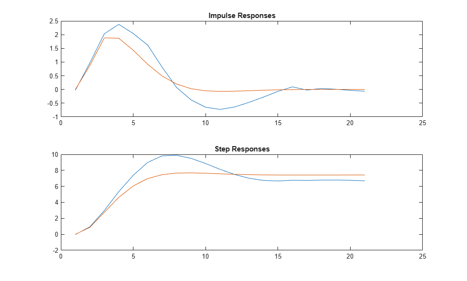
Compare a second-order ARX model's impulse response with the one obtained by correlation analysis.

load iddata1
z = z1;
ir = cra(z);
m = arx(z,[2 2 1]);
imp = [1;zeros(20,1)];
irth = sim(m,imp);
subplot(211)
plot([ir irth])
title('Impulse Responses')
subplot(212)
plot([cumsum(ir),cumsum(irth)])
title('Step Responses')

Input Arguments

collapse all

Uniformly sampled estimation data for a single experiment, specified as a SISO timetable, comma-separated matrix pair, or data object.

Timetable

Specify data as a timetable that uses a regularly spaced time vector. data can contain multiple variables representing input and output channels, but you must select a single input and output channel when estimating with cra. Use the InputName and OutputName name-value arguments to specify the input and output to use.

Comma-Separated Matrix Pair

Specify data as a comma-separated pair of single-column matrices u,y of length Ns that contain uniformly sampled input and output time-domain signal values. Here Ns is the number of samples.

Matrix-based data provides no sample-time information. The software assumes that the sample time is one second.

Data Object

Specify data as an iddata object that contains uniformly sampled input and output values. The data object must contain single-experiment time-domain data for a single-input single-output experiment. For the multivariate case, apply cra iteratively to two signals at a time or use impulseest.

For more information about working with estimation data types, see Data Domains and Data Types in System Identification Toolbox.

Number of lags for which the covariance/correlation functions are computed, specified as a positive integer. The software computes these functions from -M to M so that the length of R is 2M+1. The impulse response is computed from 0 to M.

Order of AR model to which the input is fitted, specified as a positive integer or 0.

  • To specify data prewhitening, set na to the desired order of the AR model.

  • To obtain the covariance and correlation functions of the original data sequences, set na to 0

Plot display control, specified as 1, 2, or 0, which result in the following display options:

  • 1 — Plot the estimated impulse response with a 99% confidence region.

  • 2 — Plot all the covariance functions.

  • 0 — Display no plots.

Name-Value Arguments

Specify optional pairs of arguments as Name1=Value1,...,NameN=ValueN, where Name is the argument name and Value is the corresponding value. Name-value arguments must appear after other arguments, but the order of the pairs does not matter.

Example: sys = cra(data,InputName="u2") specifies timetable variable u2 as the input variable. Alternatively, you can use sys = cra('InputName',"u2").

Input channel name, specified as a string or a character vector.

If you are using a timetable for the data source, the name in InputName must be a subset of the timetable variables.

Example: sys = cra(data,__,'InputName', "u2") selects the variable u2 as the input channel from the timetable data to use for the estimation.

Output channel name, specified as a string or character vector.

If you are using a timetable for the data source, the name in OutputName must be a subset of the timetable variables.

Example: sys = cra(data,__,'OutputName',"y3") selects the variable y3 as the output channel from the timetable data to use for the estimation.

Output Arguments

collapse all

Estimated impulse response, returned as a column vector with length equal to the number of lags specified by M. The first entry in ir corresponds to a lag of 0. Negative lags are excluded in ir.

Covariance and correlation information, returned as a (2M+1)-by-4 matrix that contains the information as shown in the following columns:

  1. Lag indices

  2. Covariance function of the output

  3. Covariance function of the input

  4. Correlation function

The input/output data that R is based on can be the original input/output data or the prewhitened data, as specified by the value of na.

You can redisplay the function plots by using the command cra(R).

99% significance level for the impulse response, returned as a numeric scalar.

Algorithms

The cra command estimates the impulse response by performing the following steps:

  1. Compute an autoregressive model for the input u as A(q)u(t)=e(t), where e is uncorrelated (white) noise, q is the time-shift operator, and A(q) is a polynomial of order na.

  2. Filter both u and the output y with A(q) to obtain the prewhitened data.

  3. Compute the covariance functions of the prewhitened u and y data and the cross-correlation function between them.

  4. Plot the functions with 99% confidence levels.

  5. Scale the correlation function to correspond to an impulse of height 1/T and duration T , where T is the sample time of the data, so that the scaled function represents an estimate of the system impulse response, and return this function in the ir output argument.

Positive values of the lag variable correspond to an influence from u to later values of y. In other words, significant correlation for negative lags is an indication of feedback from y to u in the data. The first entry of the impulse response ir corresponds to lag zero. ir excludes negative lags.

Version History

Introduced before R2006a

expand all

See Also

| | |