Main Content

spa

Estimate frequency response with fixed frequency resolution using spectral analysis

Description

example

G = spa(data) estimates the frequency response, along with uncertainty, and the noise spectrum from time- or frequency-domain data data.

data contains time-domain or frequency-domain input/output data or time series data. data can be in the form of a timetable, a comma-separated pair of numeric matrices, an iddata object,or an idfrd object that can contain complex values.

If data is a time series, that is, contains no inputs, then spa(data) returns the output power spectrum along with the uncertainty. spa computes the spectra at 128 equally spaced frequency values between 0 (excluded) and π, using a Hann window.

If data is in the form of a timetable, the software interprets the last variable is the single output variable. To change this interpretation, use the InputName and OutputName name variable arguments.

example

G = spa(data,winSize,freq) estimates the frequency response at the frequencies contained in freq, using a Hann window with size winSize.

G = spa(data,winSize,freq,maxSize) splits the input/output data into segments, each segment containing fewer than maxSize elements. Use this syntax to improve computational performance.

sys = spa(___,Name,Value) uses additional model options specified by one or more name-value arguments.

For example, specify the input and output signal variable names using sys = spa(data,'InputName',["u1","u3"],'OutputName',["y1","y4"]).

You can use this syntax with any of the previous input-argument combinations.

Examples

collapse all

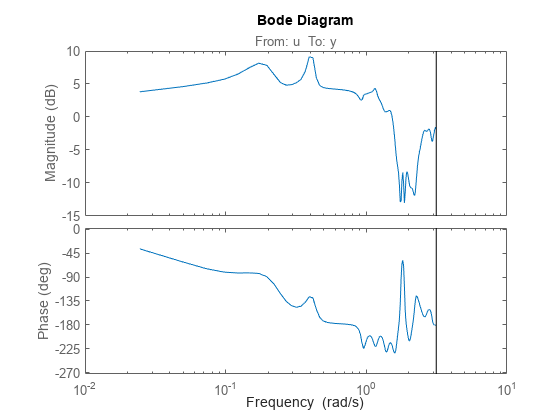
Estimate the frequency response for the input/output data in the timetable tt3. Use the default fixed resolution of 128 equally spaced logarithmic frequency values between 0 (excluded) and π.

load sdata3 tt3; 
g = spa(tt3); 
bode(g)

Figure contains 2 axes objects. Axes object 1 with title From: u To: y, ylabel Magnitude (dB) contains an object of type line. This object represents g. Axes object 2 with ylabel Phase (deg) contains an object of type line. This object represents g.

Generate the logarithmically spaced vector f.

f = logspace(-2,pi,128);

Estimate the frequency response for the input/output data in matrices umat3 and ymat3. Specify the window size as [] to obtain the default lag window size.

load sdata3 umat3 ymat3;
g = spa(umat3,ymat3,[],f);

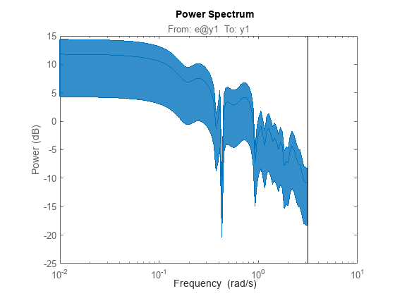
Plot the Bode response and disturbance spectrum with a confidence interval of 3 standard deviations.

h = bodeplot(g);
showConfidence(h,3)

Figure contains 2 axes objects. Axes object 1 with title From: u1 To: y1, ylabel Magnitude (dB) contains an object of type line. This object represents g. Axes object 2 with ylabel Phase (deg) contains an object of type line. This object represents g.

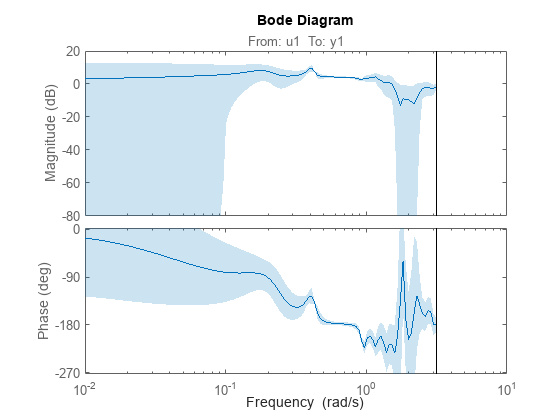
figure
h = spectrumplot(g);
showConfidence(h,3)

Figure contains an axes object. The axes object with title From: e@y1 To: y1, ylabel Power (dB) contains an object of type line. This object represents g.

Input Arguments

collapse all

Uniformly sampled estimation data, specified as a timetable, comma-separated matrix pair, or data object, as the following sections describe.

Timetable

Specify data as a timetable that uses a regularly spaced time vector. data contains variables representing input and output channels.

When you use timetables for estimation, you can use all the variables or specify a subset of channels to use.

For multiexperiment data, specify data as an Ne-by-1 cell array of timetables, where Ne is the number of experiments. The sample times of all the experiments must match.

To select individual input and output channels to use for estimation, use the InputName and OutputName name-value arguments.

For time series data, either specify data as a single-variable timetable containing only an output variable, or use InputName and OutputName name-value arguments to specify only output variables for estimation.

For example, sys = spa(data,'OutputName',"y2",'InputName',[]) estimates the time series model sys from the timetable data using the output variable y2 and no input variables.

Comma-Separated Matrix Pair

Specify data as a comma-separated pair of matrices u,y that contain uniformly sampled input and output time-domain signal values. Matrix-based data provides no sample-time information. The software assumes that the sample time is one second. Using matrix-based data for continuous-time systems is not recommended.

For SISO systems, specify u,y as column vectors with a length of Ns, where Ns is the number of samples.

For MIMO systems, specify u,y as a matrix pair with the following dimensions:

  • uNs-by-Nu, where Nu is the number of inputs

  • yNs-by-Ny, where Ny is the number of outputs

For multiexperiment data, specify u,y as a pair of 1-by-Ne cell arrays, where Ne is the number of experiments.

For time series systems, specify an empty u, that is, [],y.

Data Object

An estimation data object, specified as a time-domain or frequency-domain iddata object or an idfrd object that contains uniformly sampled input and output values. The data object can have one or more output channels and zero or more input channels. By default, the software sets the sample time of the model to the sample time of the estimation data.

For more information about working with estimation data types, see Data Domains and Data Types in System Identification Toolbox.

Hann window size, also known as lag size, specified as a scalar integer. By default, the function sets the window size to min(length(data)/10,30).

Frequencies at which to estimate spectral response, specified as a row vector in units of rad/TimeUnit, where TimeUnit refers to the TimeUnit property of data. By default, the function sets freq to a vector of 128 values in the range (0,π], evenly spaced logarithmically. For discrete-time models, set freq within the Nyquist frequency bound.

Maximum size of segments within data, specified as a positive integer. If you omit this argument, the function performs estimation using the full data set in data rather than segmenting the data.

Name-Value Arguments

Specify optional pairs of arguments as Name1=Value1,...,NameN=ValueN, where Name is the argument name and Value is the corresponding value. Name-value arguments must appear after other arguments, but the order of the pairs does not matter.

Before R2021a, use commas to separate each name and value, and enclose Name in quotes.

Example: sys = spa(data,'InputName',"u2")

Input channel names, specified as a string, character vector, string array, or cell array of character vectors.

If you are using a timetable for the data source, the names in InputName must be a subset of the timetable variables.

Example: sys = spa(tt,__,'InputName',["u1" "u2"]) selects the variables u1 and u2 as the input channels from the timetable tt to use for the estimation.

Output channel names, specified as a string, character vector, string array, or cell array of character vectors.

If you are using a timetable for the data source, the names in OutputName must be a subset of the timetable variables.

Example: sys = spa(tt,__,'OutputName',["y1" "y3"]) selects the variables y1 and y3 as the output channels from the timetable tt to use for the estimation.

Output Arguments

collapse all

Frequency response with uncertainty and noise spectrum, specified as an idfrd object. For time series data, G is the estimated spectrum and standard deviation.

Information about the estimation results and options used is stored in the Report property of the model. Report has the following fields.

Report FieldDescription
Status

Summary of the model status, which indicates whether the model was created by construction or obtained by estimation.

Method

Estimation command used.

windowSize

Size of the Hann window.

DataUsed

Attributes of the data used for estimation. Structure with the following fields.

FieldDescription
Name

Name of the data set.

Type

Data type.

Length

Number of data samples.

Ts

Sample time. This is equivalent to data.Ts.

InterSample

Input intersample behavior. One of the following values:

  • 'zoh' — Zero-order hold maintains a piecewise-constant input signal between samples.

  • 'foh' — First-order hold maintains a piecewise-linear input signal between samples.

  • 'bl' — Band-limited behavior specifies that the continuous-time input signal has zero power above the Nyquist frequency.

The value of InterSample has no effect on estimation results for discrete-time models.

InputOffset

Offset removed from time-domain input data during estimation.

OutputOffset

Offset removed from time-domain output data during estimation.

More About

collapse all

Frequency Response Function

A frequency response function describes the steady-state response of a system to sinusoidal inputs. For a linear system, a sinusoidal input of a specific frequency results in an output that is also a sinusoid with the same frequency, but with a different amplitude and phase. The frequency response function describes the amplitude change and phase shift as a function of frequency.

To better understand the frequency response function, consider the following description of a linear dynamic system:

y(t)=G(q)u(t)+v(t)

Here, u(t) and y(t) are the input and output signals, respectively. G(q) is called the transfer function of the system—it captures the system dynamics that take the input to the output. The notation G(q)u(t) represents the following operation:

G(q)u(t)=k=1g(k)u(tk)

q is the shift operator, defined by the following equation:

G(q)=k=1g(k)qk      q1u(t)=u(t1)

G(q) is the frequency-response function when it is evaluated on the unit circle, G(q=e).

Together, G(q=e) and the output noise spectrum Φ^v(ω) compose the frequency-domain description of the system.

The frequency-response function estimated using the Blackman-Tukey approach is given by the following equation:

G^N(eiω)=Φ^yu(ω)Φ^u(ω)

In this case, ^ represents approximate quantities. For a derivation of this equation, see the chapter on nonparametric time- and frequency-domain methods in [1].

Output Noise Spectrum

The output noise spectrum (spectrum of v(t)) is given by the following equation:

Φ^v(ω)=Φ^y(ω)|Φ^yu(ω)|2Φ^u(ω)

This equation for the noise spectrum is derived by assuming that the linear relationship y(t)=G(q)u(t)+v(t) holds, that u(t) is independent of v(t), and that the following relationships between the spectra hold:

Φy(ω)=|G(eiω)|2Φu(ω)+Φv(ω)

Φyu(ω)=G(eiω)Φu(ω)

Here, the noise spectrum is given by the following equation:

Φv(ω)τ=Rv(τ)eiwτ

Φ^yu(ω) is the output-input cross-spectrum and Φ^u(ω) is the input spectrum.

Alternatively, the disturbance v(t) can be described as filtered white noise:

v(t)=H(q)e(t)

Here, e(t) is the white noise with variance λ and the noise power spectrum is given by the following equation:

Φv(ω)=λ|H(eiω)|2

Algorithms

spa applies the Blackman-Tukey spectral analysis method by following these steps:

  1. Compute the covariances and cross-covariance from u(t) and y(t):

    R^y(τ)=1Nt=1Ny(t+τ)y(t)R^u(τ)=1Nt=1Nu(t+τ)u(t)R^yu(τ)=1Nt=1Ny(t+τ)u(t)

  2. Compute the Fourier transforms of the covariances and the cross-covariance:

    Φ^y(ω)=τ=MMR^y(τ)WM(τ)eiωτΦ^u(ω)=τ=MMR^u(τ)WM(τ)eiωτΦ^yu(ω)=τ=MMR^yu(τ)WM(τ)eiωτ

    where WM(τ) is the Hann window with a width (lag size) of M. You can specify M to control the frequency resolution of the estimate, which is approximately equal to 2π/M rad/sample time.

    By default, this operation uses 128 equally spaced frequency values between 0 (excluded) and π, where w = [1:128]/128*pi/Ts and Ts is the sample time of that data set. The default lag size of the Hann window is M = min(length(data)/10,30). For default frequencies, the operation uses fast Fourier transforms (FFT), which are more efficient than for user-defined frequencies.

    Note

    M = γ is in Table 6.1 of [1]. Standard deviations are on pages 184 and 188 in [1].

  3. Compute the frequency-response function G^N(eiω) and the output noise spectrum Φ^v(ω).

    G^N(eiω)=Φ^yu(ω)Φ^u(ω)

    Φv(ω)τ=Rv(τ)eiwτ

spectrum is the spectrum matrix for both the output and the input channels. That is, if z = [data.OutputData, data.InputData], spectrum contains as spectrum data the matrix-valued power spectrum of z.

S=m=MMEz(t+m)z(t)WM(Ts)exp(iωm)

Here, ' is a complex-conjugate transpose.

References

[1] Ljung, Lennart. System Identification: Theory for the User. 2nd ed. Prentice Hall Information and System Sciences Series. Upper Saddle River, NJ: Prentice Hall PTR, 1999.

Version History

Introduced before R2006a

expand all