fevd

Generate vector autoregression (VAR) model forecast error variance decomposition (FEVD)

Since R2019a

Syntax

Decomposition = fevd(Mdl)

Decomposition = fevd(Mdl,Name=Value)

[Decomposition,Lower,Upper] = fevd(___)

Tbl = fevd(___)

Description

The fevd function returns the forecast error variance decomposition (FEVD) of the variables in a VAR(p) model attributable to shocks to each response variable in the system. A fully specified varm model object characterizes the VAR model.

To estimate or plot the FEVD of a dynamic linear model characterized by structural, autoregression, or moving average coefficient matrices, see armafevd.

The FEVD provides information about the relative importance of each innovation in affecting the forecast error variance of all response variables in the system. In contrast, the impulse response function (IRF) traces the effects of an innovation shock to one variable on the response of all variables in the system. To estimate the IRF of a VAR model characterized by a varm model object, see irf.

You can supply optional data, such as a presample, as a numeric array, table, or timetable. However, all specified input data must be the same data type. When the input model is estimated (returned by estimate), supply the same data type as the data used to estimate the model. The data type of the outputs matches the data type of the specified input data.

Decomposition = fevd(Mdl) returns a numeric array containing the orthogonalized FEVDs of the response variables that compose the VAR(p) model Mdl, characterized by a fully specified varm model object. fevd shocks variables at time 0, and returns the FEVD for times 1 through 20.

If Mdl is an estimated model (returned by estimate) fit to a numeric matrix of input response data, this syntax applies.

Decomposition = fevd(Mdl,Name=Value) uses additional options specified by one or more name-value arguments. fevd returns numeric arrays when all optional input data are numeric arrays. For example, fevd(Mdl,NumObs=10,Method="generalized") specifies estimating a generalized FEVD for periods 1 through 10.

If Mdl is an estimated model fit to a numeric matrix of input response data, this syntax applies.

[Decomposition,Lower,Upper] = fevd(___) returns numeric arrays of lower Lower and upper Upper 95% confidence bounds for confidence intervals on the true FEVD, for each period and variable in the FEVD, using any input argument combination in the previous syntaxes. By default, fevd estimates confidence bounds by conducting Monte Carlo simulation.

If Mdl is an estimated model fit to a numeric matrix of input response data, this syntax applies.

If Mdl is a custom varm model object (an object not returned by estimate or modified after estimation), fevd can require a sample size for the simulation SampleSize or presample responses Y0.

Tbl = fevd(___) returns the table or timetable Tbl containing the FEVDs and, optionally, corresponding 95% confidence bounds, of the response variables that compose the VAR(p) model Mdl. The FEVD of the corresponding response is a variable in Tbl containing a matrix with columns corresponding to the variables in the system shocked at time 0. (since R2022b)

If you set at least one name-value argument that controls the 95% confidence bounds on the FEVD, Tbl also contains a variable for each of the lower and upper bounds. For example, Tbl contains confidence bounds when you set the NumPaths name-value argument.

If Mdl is an estimated model fit to a table or timetable of input response data, this syntax applies.

Examples

Specify Data in Numeric Matrix When Plotting FEVD

Fit a 4-D VAR(2) model to Danish money and income rate series data in a numeric matrix. Then, estimate and plot the orthogonalized FEVD from the estimated model.

Load the Danish money and income data set.

load Data_JDanish

For more details on the data set, enter Description at the command line.

Assuming that the series are stationary, create a varm model object that represents a 4-D VAR(2) model. Specify the variable names.

Mdl = varm(4,2);
Mdl.SeriesNames = DataTable.Properties.VariableNames;

Mdl is a varm model object specifying the structure of a 4-D VAR(2) model; it is a template for estimation.

Fit the VAR(2) model to the numeric matrix of time series data Data.

EstMdl = estimate(Mdl,Data);

EstMdl is a fully specified varm model object representing an estimated 4-D VAR(2) model.

Estimate the orthogonalized FEVD from the estimated VAR(2) model.

Decomposition = fevd(EstMdl);

Decomposition is a 20-by-4-by-4 array representing the FEVD of Mdl. Rows correspond to consecutive time points from time 1 to 20, columns correspond to variables receiving a one-standard-deviation innovation shock at time 0, and pages correspond to the variables whose forecast error variance fevd decomposes. Mdl.SeriesNames specifies the variable order.

Because Decomposition represents an orthogonalized FEVD, rows should sum to 1. This characteristic illustrates that orthogonalized FEVDs represent proportions of variance contributions. Confirm that all rows of Decomposition sum to 1.

rowsums = sum(Decomposition,2);
sum((rowsums - 1).^2 > eps)

ans = 
ans(:,:,1) =

     0


ans(:,:,2) =

     0


ans(:,:,3) =

     0


ans(:,:,4) =

     0

Row sums among the pages are close to 1.

Display the contributions to the forecast error variance of the bond rate when real income is shocked at time 0.

Decomposition(:,2,3)

ans = 20×1

    0.0499
    0.1389
    0.1700
    0.1807
    0.1777
    0.1694
    0.1601
    0.1516
    0.1446
    0.1390
      ⋮

Plot the FEVDs of all series on separate plots by passing the estimated AR coefficient matrices and innovations covariance matrix of Mdl to armafevd.

armafevd(EstMdl.AR,[],"InnovCov",EstMdl.Covariance);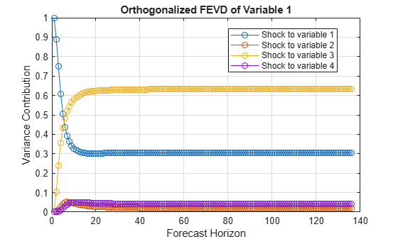

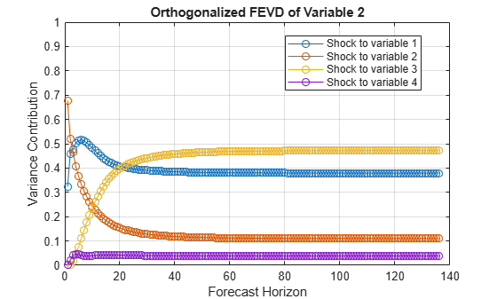
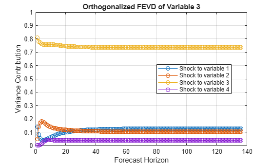
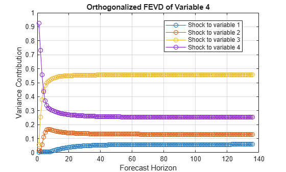
Each plot shows the four FEVDs of a variable when all other variables are shocked at time 0. Mdl.SeriesNames specifies the variable order.

Estimate Generalized FEVD of VAR Model

Consider the 4-D VAR(2) model in Specify Data in Numeric Matrix When Plotting FEVD. Estimate the generalized FEVD of the system for 100 periods.

Load the Danish money and income data set, and then estimate the VAR(2) model.

load Data_JDanish

Mdl = varm(4,2);
Mdl.SeriesNames = DataTable.Properties.VariableNames;
Mdl = estimate(Mdl,DataTable.Series);

Estimate the generalized FEVD from the estimated VAR(2) model over a forecast horizon with length 100.

Decomposition = fevd(Mdl,Method="generalized",NumObs=100);

Decomposition is a 100-by-4-by-4 array representing the generalized FEVD of Mdl.

Plot the generalized FEVD of the bond rate when real income is shocked at time 0.

figure;
plot(1:100,Decomposition(:,2,3))
title("FEVD of IB When Y Is Shocked")
xlabel("Forecast Horizon")
ylabel("Variance Contribution")
grid on

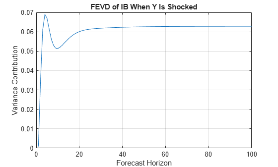
When real income is shocked, the contribution of the bond rate to the forecast error variance settles at approximately 0.061.

Specify Data in Timetables When Computing FEVD and Confidence Intervals

Since R2022b

Fit a 4-D VAR(2) model to Danish money and income rate series data in a timetable. Then, estimate and plot the orthogonalized FEVD and corresponding confidence intervals from the estimated model.

Load the Danish money and income data set.

load Data_JDanish

The data set includes four time series in the timetable DataTimeTable. For more details on the data set, enter Description at the command line.

Assuming that the series are stationary, create a varm model object that represents a 4-D VAR(2) model. Specify the variable names.

Mdl = varm(4,2);
Mdl.SeriesNames = DataTimeTable.Properties.VariableNames;

Mdl is a varm model object specifying the structure of a 4-D VAR(2) model; it is a template for estimation.

Fit the VAR(2) model to the data set.

EstMdl = estimate(Mdl,DataTimeTable);

Mdl is a fully specified varm model object representing an estimated 4-D VAR(2) model.

Estimate the orthogonalized FEVD and corresponding 95% confidence intervals from the estimated VAR(2) model. To return confidence intervals, you must set a name-value argument that controls confidence intervals, for example, Confidence. Set Confidence to 0.95.

rng(1); % For reproducibility
Tbl = fevd(EstMdl,Confidence=0.95);
size(Tbl)

ans = 1×2

    20    12

Tbl is a timetable with 20 rows, representing the periods in the FEVD, and 12 variables. Each variable is a 20-by-4 matrix of the FEVD or confidence bound associated with a variable in the model EstMdl. For example, Tbl.M2_FEVD(:,2) is the FEVD of M2 resulting from a one-standard-deviation shock on 01-Apr-1974 (period 0) to Mdl.SeriesNames(2), which is the variable Y. [Tbl.M2_FEVD_LowerBound(:,2),Tbl.M2_FEVD_UpperBound(:,2)] are the corresponding 95% confidence intervals.

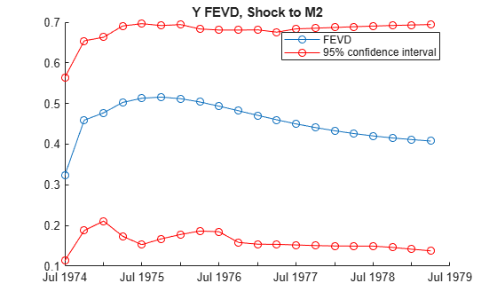
Plot the FEVD of M2 and its 95% confidence interval resulting from a one-standard-deviation shock on 01-Apr-1974 (period 0) to Mdl.SeriesNames(2), which is the variable Y.

idxM2 = startsWith(Tbl.Properties.VariableNames,"M2");
M2FEVD = Tbl(:,idxM2);
shockIdx = 2;
figure
hold on
plot(M2FEVD.Time,M2FEVD.M2_FEVD(:,shockIdx),"-o")
plot(M2FEVD.Time,[M2FEVD.M2_FEVD_LowerBound(:,shockIdx) ...
    M2FEVD.M2_FEVD_UpperBound(:,shockIdx)],"-o",Color="r")
legend("FEVD","95% confidence interval")
title('M2 FEVD, Shock to Y')
hold off

Monte Carlo Confidence Intervals on True FEVD

Consider the 4-D VAR(2) model in Specify Data in Numeric Matrix When Plotting FEVD. Estimate and plot its orthogonalized FEVD and 95% Monte Carlo confidence intervals on the true FEVD.

Load the Danish money and income data set, and then estimate the VAR(2) model.

load Data_JDanish

Mdl = varm(4,2);
Mdl.SeriesNames = DataTable.Properties.VariableNames;
Mdl = estimate(Mdl,DataTable.Series);

Estimate the FEVD and corresponding 95% Monte Carlo confidence intervals from the estimated VAR(2) model.

rng(1); % For reproducibility
[Decomposition,Lower,Upper] = fevd(Mdl);

Decomposition, Lower, and Upper are 20-by-4-by-4 arrays representing the orthogonalized FEVD of Mdl and corresponding lower and upper bounds of the confidence intervals. For all arrays, rows correspond to consecutive time points from time 1 to 20, columns correspond to variables receiving a one-standard-deviation innovation shock at time 0, and pages correspond to the variables whose forecast error variance fevd decomposes. Mdl.SeriesNames specifies the variable order.

Plot the orthogonalized FEVD with its confidence bounds of the bond rate when real income is shocked at time 0.

fevdshock2resp3 = Decomposition(:,2,3);
FEVDCIShock2Resp3 = [Lower(:,2,3) Upper(:,2,3)];

figure;
h1 = plot(1:20,fevdshock2resp3);
hold on
h2 = plot(1:20,FEVDCIShock2Resp3,'r--');
legend([h1 h2(1)],["FEVD" "95% confidence interval"], ...
    'Location',"best")
xlabel("Forecast Horizon");
ylabel("Variance Contribution");
title("FEVD of IB When Y Is Shocked");
grid on
hold off

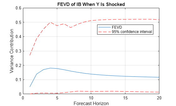
In the long run, and when real income is shocked, the proportion of forecast error variance of the bond rate settles between approximately 0 and 0.5 with 95% confidence.

Bootstrap Confidence Intervals on True FEVD

Consider the 4-D VAR(2) model in Specify Data in Numeric Matrix When Plotting FEVD. Estimate and plot its orthogonalized FEVD and 90% bootstrap confidence intervals on the true FEVD.

Load the Danish money and income data set, and then estimate the VAR(2) model. Return the residuals from model estimation.

load Data_JDanish

Mdl = varm(4,2);
Mdl.SeriesNames = DataTable.Properties.VariableNames;
[Mdl,~,~,Res] = estimate(Mdl,DataTable.Series);
T = size(DataTable,1) % Total sample size

T = 55

n = size(Res,1)         % Effective sample size

n = 53

Res is a 53-by-4 array of residuals. Columns correspond to the variables in Mdl.SeriesNames. The estimate function requires Mdl.P = 2 observations to initialize a VAR(2) model for estimation. Because presample data (Y0) is unspecified, estimate takes the first two observations in the specified response data to initialize the model. Therefore, the resulting effective sample size is T – Mdl.P = 53, and rows of Res correspond to the observation indices 3 through T.

Estimate the orthogonalized FEVD and corresponding 90% bootstrap confidence intervals from the estimated VAR(2) model. Draw 500 paths of length n from the series of residuals.

rng(1); % For reproducibility
[Decomposition,Lower,Upper] = fevd(Mdl,E=Res,NumPaths=500, ...
    Confidence=0.9);

Plot the orthogonalized FEVD with its confidence bounds of the bond rate when real income is shocked at time 0.

fevdshock2resp3 = Decomposition(:,2,3);
FEVDCIShock2Resp3 = [Lower(:,2,3) Upper(:,2,3)];

figure;
h1 = plot(0:19,fevdshock2resp3);
hold on
h2 = plot(0:19,FEVDCIShock2Resp3,"r--");
legend([h1 h2(1)],["FEVD" "90% confidence interval"], ...
    'Location',"best")
xlabel("Time Index");
ylabel("Response");
title("FEVD of IB When Y Is Shocked");
grid on
hold off

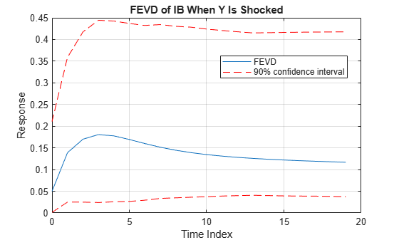
In the long run, and when real income is shocked, the proportion of forecast error variance of the bond rate settles between approximately 0.05 and 0.4 with 90% confidence.

Input Arguments

Mdl — VAR model

varm model object

VAR model, specified as a varm model object created by varm or estimate. Mdl must be fully specified.

If Mdl is an estimated model (returned by estimate) , you must supply any optional data using the same data type as the input response data, to which the model is fit.

If Mdl is a custom varm model object (an object not returned by estimate or modified after estimation), fevd can require a sample size for the simulation SampleSize or presample responses Y0.

Name-Value Arguments

Specify optional pairs of arguments as Name1=Value1,...,NameN=ValueN, where Name is the argument name and Value is the corresponding value. Name-value arguments must appear after other arguments, but the order of the pairs does not matter.

Before R2021a, use commas to separate each name and value, and enclose Name in quotes.

Example: fevd(Mdl,NumObs=10,Method="generalized",E=Res) specifies estimating a generalized FEVD for periods 1 through 10, and bootstraps the residuals in the numeric array Res to compute the 95% confidence bounds.

Options for All FEVDs

NumObs — Number of periods

20 (default) | positive integer

Number of periods for which fevd computes the FEVD (the forecast horizon), specified as a positive integer. NumObs specifies the number of observations to include in the FEVD (the number of rows in Decomposition).

Example: NumObs=10 specifies estimation of the FEVD for times 1 through 10.

Data Types: double

Method — FEVD computation method

"orthogonalized" (default) | "generalized" | character vector

FEVD computation method, specified as a value in this table.

Value	Description
"orthogonalized"	Compute variance decompositions using orthogonalized, one-standard-deviation innovation shocks. fevd uses the Cholesky factorization of Mdl.Covariance for orthogonalization.
"generalized"	Compute variance decompositions using one-standard-deviation innovation shocks.

Example: Method="generalized"

Data Types: char | string

Options for Confidence Bound Estimation

NumPaths — Number of sample paths

100 (default) | positive integer

Number of sample paths (trials) to generate, specified as a positive integer.

Example: NumPaths=1000 generates 1000 sample paths from which the software derives the confidence bounds.

Data Types: double

SampleSize — Number of observations for Monte Carlo simulation or bootstrap per sample path

positive integer

Number of observations for the Monte Carlo simulation or bootstrap per sample path, specified as a positive integer.

• If Mdl is an estimated varm model object (an object returned by estimate and unmodified thereafter), the default is the sample size of the data to which the model is fit (see summarize).

• Otherwise:

  • If fevd estimates confidence bounds by conducting a Monte Carlo simulation, you must specify SampleSize.

  • If fevd estimates confidence bounds by bootstrapping residuals, the default is the length of the specified series of residuals (size(Res,1), where Res is the number of residuals in E or InSample).

Example: If you specify SampleSize=100 and do not specify the E name-value argument, the software estimates confidence bounds from NumPaths random paths of length 100 from Mdl.

Example: If you specify SampleSize=100,E=Res, the software resamples, with replacement, 100 observations (rows) from Res to form a sample path of innovations to filter through Mdl. The software forms NumPaths random sample paths from which it derives confidence bounds.

Data Types: double

Y0 — Presample response data

numeric matrix

Presample response data that provides initial values for model estimation during the simulation, specified as a numpreobs-by-numseries numeric matrix. Use Y0 only in the following situations:

• You supply other optional data inputs as numeric matrices.

• Mdl is an estimated varm model object (an object returned by estimate and unmodified thereafter) fit to a numeric matrix of response data.

numpreobs is the number of presample observations. numseries is Mdl.NumSeries, the dimensionality of the input model.

Each row is a presample observation, and measurements in each row occur simultaneously. The last row contains the latest presample observation. numpreobs is the number of specified presample responses and it must be at least Mdl.P. If you supply more rows than necessary, fevd uses the latest Mdl.P observations only.

numseries is the dimensionality of the input VAR model Mdl.NumSeries. Columns must correspond to the response variables in Mdl.SeriesNames.

The following situations determine the default or whether presample response data is required.

• If Mdl is an unmodified estimated model, fevd sets Y0 to the presample response data used for estimation by default (see the Y0 name-value argument of estimate).

• If Mdl is a custom model and you return confidence bounds Lower or Upper, you must specify Y0.

Data Types: double

Presample — Presample data

table | timetable

Since R2022b

Presample data that provides initial values for the model Mdl, specified as a table or timetable with numprevars variables and numpreobs rows. Use Presample only in the following situations:

• You supply other optional data inputs as tables or timetables.

• Mdl is an estimated varm model object (an object returned by estimate and unmodified thereafter) fit to response data in a table or timetable.

Each row is a presample observation, and measurements in each row occur simultaneously. numpreobs must be at least Mdl.P. If you supply more rows than necessary, fevd uses the latest Mdl.P observations only.

Each variable is a numpreobs numeric vector representing one path. To control presample variable selection, see the optional PresampleResponseVariables name-value argument.

If Presample is a timetable, all the following conditions must be true:

• Presample must represent a sample with a regular datetime time step (see isregular).

• The datetime vector of sample timestamps Presample.Time must be ascending or descending.

If Presample is a table, the last row contains the latest presample observation.

The following situations determine the default or whether presample response data is required.

• If Mdl is an unmodified estimated model, fevd sets Presample to the presample response data used for estimation by default (see the Presample name-value argument of estimate).

• If Mdl is a custom model (for example, you modify a model after estimation by using dot notation) and you return confidence bounds in the table or timetable Tbl, you must specify Presample.

PresampleResponseVariables — Variables to select from Presample to use for presample response data

string vector | cell vector of character vectors | vector of integers | logical vector

Since R2022b

Variables to select from Presample to use for presample data, specified as one of the following data types:

• String vector or cell vector of character vectors containing numseries variable names in Presample.Properties.VariableNames

• A length numseries vector of unique indices (integers) of variables to select from Presample.Properties.VariableNames

• A length numprevars logical vector, where PresampleResponseVariables(j) = true selects variable j from Presample.Properties.VariableNames, and sum(PresampleResponseVariables) is numseries

PresampleResponseVariables applies only when you specify Presample.

The selected variables must be numeric vectors and cannot contain missing values (NaN).

PresampleResponseNames does not need to contain the same names as in Mdl.SeriesNames; fevd uses the data in selected variable PresampleResponseVariables(j) as a presample for Mdl.SeriesNames(j).

If the number of variables in Presample matches Mdl.NumSeries, the default specifies all variables in Presample. If the number of variables in Presample exceeds Mdl.NumSeries, the default matches variables in Presample to names in Mdl.SeriesNames.

Example: PresampleResponseVariables=["GDP" "CPI"]

Example: PresampleResponseVariables=[true false true false] or PresampleResponseVariable=[1 3] selects the first and third table variables for presample data.

Data Types: double | logical | char | cell | string

X — Predictor data

numeric matrix

Predictor data x_t for estimating the model regression component during the simulation, specified as a numeric matrix containing numpreds columns. Use X only in the following situations:

• You supply other optional data inputs as numeric matrices.

• Mdl is an estimated varm model object (an object returned by estimate and unmodified thereafter) fit to a numeric matrix of response data.

numpreds is the number of predictor variables (size(Mdl.Beta,2)).

Each row corresponds to an observation, and measurements in each row occur simultaneously. The last row contains the latest observation. X must have at least SampleSize rows. If you supply more rows than necessary, fevd uses only the latest observations. fevd does not use the regression component in the presample period.

Columns correspond to individual predictor variables. All predictor variables are present in the regression component of each response equation.

To maintain model consistency when fevd estimates the confidence bounds, specify predictor data when Mdl has a regression component. If Mdl is an estimated model, specify the predictor data used during model estimation (see the X name-value argument of estimate).

By default, fevd excludes the regression component from confidence bound estimation, regardless of its presence in Mdl.

Data Types: double

E — Series of residuals e_t from which to draw bootstrap samples

numeric matrix

Series of residuals from which to draw bootstrap samples, specified as a numperiods-by-numseries numeric matrix. fevd assumes that E is free of serial correlation. Use E only in the following situations:

• You supply other optional data inputs as numeric matrices.

• Mdl is an estimated varm model object (an object returned by estimate and unmodified thereafter) fit to a numeric matrix of response data.

Each column is the residual series corresponding to the response series names in Mdl.SeriesNames.

Each row corresponds to a period in the FEVD and the corresponding confidence bounds.

If Mdl is an estimated varm model object (an object returned by estimate), you can specify E as the inferred residuals from estimation (see the E output argument of estimate or infer).

By default, fevd derives confidence bounds by conducting a Monte Carlo simulation.

Data Types: double

InSample — Time series data

table | timetable

Since R2022b

Time series data containing numvars variables, including numseries variables of residuals e_t to bootstrap or numpreds predictor variables x_t for the model regression component, specified as a table or timetable. Use InSample only in the following situations:

• You supply other optional data inputs as tables or timetables.

• Mdl is an estimated varm model object (an object returned by estimate and unmodified thereafter) fit to response data in a table or timetable.

Each variable is a single path of observations, which fevd applies to all NumPaths sample paths. If you specify Presample, you must specify which variables are residuals and predictors. See the ResidualVariables and PredictorVariables name-value arguments.

Each row is an observation, and measurements in each row occur simultaneously. InSample must have at least SampleSize rows. If you supply more rows than necessary, fevd uses only the latest observations.

If InSample is a timetable, the following conditions apply:

• InSample must represent a sample with a regular datetime time step (see isregular).

• The datetime vector InSample.Time must be ascending or descending.

• Presample must immediately precede InSample, with respect to the sampling frequency.

If InSample is a table, the last row contains the latest observation.

By default, fevd derives confidence bounds by conducting a Monte Carlo simulation and does not use the regression component, regardless of its presence in Mdl.

ResidualVariables — Variables to select from InSample to treat as residuals e_t for bootstrapping

string vector | cell vector of character vectors | vector of integers | logical vector

Since R2022b

Variables to select from InSample to treat as residuals for bootstrapping, specified as one of the following data types:

• String vector or cell vector of character vectors containing numseries variable names in InSample.Properties.VariableNames

• A length numseries vector of unique indices (integers) of variables to select from InSample.Properties.VariableNames

• A length numvars logical vector, where ResidualVariables(j) = true selects variable j from InSample.Properties.VariableNames, and sum(ResidualVariables) is numseries

Regardless, selected residual variable j is the residual series for Mdl.SeriesNames(j).

The selected variables must be numeric vectors and cannot contain missing values (NaN).

By default, fevd derives confidence bounds by conducting a Monte Carlo simulation.

Example: ResidualVariables=["GDP_Residuals" "CPI_Residuals"]

Example: ResidualVariables=[true false true false] or ResidualVariable=[1 3] selects the first and third table variables as the disturbance variables.

Data Types: double | logical | char | cell | string

PredictorVariables — Variables to select from InSample to treat as exogenous predictor variables x_t

string vector | cell vector of character vectors | vector of integers | logical vector

Since R2022b

Variables to select from InSample to treat as exogenous predictor variables x_t, specified as one of the following data types:

• String vector or cell vector of character vectors containing numpreds variable names in InSample.Properties.VariableNames

• A length numpreds vector of unique indices (integers) of variables to select from InSample.Properties.VariableNames

• A length numvars logical vector, where PredictorVariables(j) = true selects variable j from InSample.Properties.VariableNames, and sum(PredictorVariables) is numpreds

Regardless, selected predictor variable j corresponds to the coefficients Mdl.Beta(:,j).

PredictorVariables applies only when you specify InSample.

The selected variables must be numeric vectors and cannot contain missing values (NaN).

By default, fevd excludes the regression component, regardless of its presence in Mdl.

Example: PredictorVariables=["M1SL" "TB3MS" "UNRATE"]

Example: PredictorVariables=[true false true false] or PredictorVariable=[1 3] selects the first and third table variables as the response variables.

Data Types: double | logical | char | cell | string

Confidence — Confidence level

0.95 (default) | numeric scalar in [0,1]

Confidence level for the confidence bounds, specified as a numeric scalar in the interval [0,1].

For each period, randomly drawn confidence intervals cover the true response 100*Confidence% of the time.

The default value is 0.95, which implies that the confidence bounds represent 95% confidence intervals.

Example: Confidence=0.9 specifies 90% confidence intervals.

Data Types: double

Note

• NaN values in Y0, X, and E indicate missing data. fevd removes missing data from these arguments by list-wise deletion. For each argument, if a row contains at least one NaN, fevd removes the entire row.

  List-wise deletion reduces the sample size, can create irregular time series, and can cause E and X to be unsynchronized.

• fevd issues an error when any table or timetable input contains missing values.

Output Arguments

Decomposition — FEVD

numeric array

FEVD of each response variable, returned as a numobs-by-numseries-by-numseries numeric array. numobs is the value of NumObs. Columns and pages correspond to the response variables in Mdl.SeriesNames.

fevd returns Decomposition only in the following situations:

• You supply optional data inputs as numeric matrices.

• Mdl is an estimated model fit to a numeric matrix of response data.

Decomposition(t,j,k) is the contribution to the variance decomposition of variable k attributable to a one-standard-deviation innovation shock to variable j at time t, for t = 1,2,…,numobs, j = 1,2,...,numseries, and k = 1,2,...,numseries.

Lower — Lower confidence bounds

numeric array

Lower confidence bounds, returned as a numobs-by-numseries-by-numseries numeric array. Elements of Lower correspond to elements of Decomposition.

fevd returns Lower only in the following situations:

• You supply optional data inputs as numeric matrices.

• Mdl is an estimated model fit to a numeric matrix of response data.

Lower(t,j,k) is the lower bound of the 100*Confidence-th percentile interval on the true contribution to the variance decomposition of variable k attributable to a one-standard-deviation innovation shock to variable j at time 0.

Upper — Upper confidence bounds

numeric array

Upper confidence bounds, returned as a numobs-by-numseries-by-numseries numeric array. Elements of Upper correspond to elements of Decomposition.

fevd returns Upper only in the following situations:

• You supply optional data inputs as numeric matrices.

• Mdl is an estimated model fit to a numeric matrix of response data.

Upper(t,j,k) is the upper bound of the 100*Confidence-th percentile interval on the true contribution to the variance decomposition of variable k attributable to a one-standard-deviation innovation shock to variable j at time 0.

Tbl — FEVD and confidence bounds

table | timetable

Since R2022b

FEVD and confidence bounds, returned as a table or timetable with numobs rows. fevd returns Tbl only in the following situations:

• You supply optional data inputs as tables or timetables.

• Mdl is an estimated model object fit to response data in a table or timetable.

Regardless, the data type of Tbl is the same as the data type of specified data.

Tbl contains the following variables:

• The FEVD of each series in y_t. Each FEVD variable in Tbl is a numobs-by-numseries numeric matrix, where numobs is the value of NumObs and numseries is the value of Mdl.NumSeries. fevd names the FEVD of response variable ResponseJ in Mdl.SeriesNames ResponseJ_FEVD. For example, if Mdl.Series(j) is GDP, Tbl contains a variable for the corresponding FEVD with the name GDP_FEVD.

  ResponseJ_FEVD(t,k) is the contribution to the variance decomposition of response variable ResponseJ attributable to a one-standard-deviation innovation shock to variable k at time t, for t = 1,2,…,numobs, J = 1,2,...,numseries, and k = 1,2,...,numseries.

• The lower and upper confidence bounds on the true FEVD of the response series, when you set at least one name-value argument that controls the confidence bounds. Each confidence bound variable in Tbl is a numobs-by-numseries numeric matrix. ResponseJ_FEVD_LowerBound and ResponseJ_FEVD_UpperBound are the names of the lower and upper bound variables, respectively, of the confidence interval on the FEVD of response variable Mdl.SeriesNames(J) = ResponseJ. For example, if Mdl.SeriesNames(j) is GDP, Tbl contains variables for the corresponding lower and upper bounds of the confidence interval with the name GDP_FEVD_LowerBound and GDP_FEVD_UpperBound.

  (ResponseJ_FEVD_LowerBound(t,k), ResponseJ_FEVD_UpperBound(t,k)) is the 95% confidence interval on the FEVD of response variable ResponseJ attributable to a one-standard-deviation innovation shock to variable k at time t, for t = 1,2,…,numobs, J = 1,2,...,numseries, and k = 1,2,...,numseries.

If Tbl is a timetable, the row order of Tbl, either ascending or descending, matches the row order of InSample, when you specify it. If you do not specify InSample and you specify Presample, the row order of Tbl is the same as the row order Presample.

More About

Forecast Error Variance Decomposition

The forecast error variance decomposition (FEVD) of a multivariate, dynamic system shows the relative importance of a shock to each innovation in affecting the forecast error variance of all variables in the system.

Consider a numseries-D VAR(p) model for the multivariate response variable y_t. In lag operator notation, the infinite lag MA representation of y_t is

$$\begin{array}{c}{y}_t={\Phi }^{-1}(L)\left(c+\beta x_t+\delta t\right)+{\Phi }^{-1}(L){\epsilon }_t\\ =\Omega (L)\left(c+\beta x_t+\delta t\right)+\Omega (L){\epsilon }_t.\end{array}$$

The general form of the FEVD of y_kt (variable k) m periods into the future, attributable to a one-standard-deviation innovation shock to y_jt, is

$${\gamma }_{mjk}=\frac{{\displaystyle \sum _{t=0}^{m-1}{\left(e_k{}^{\prime }{C}_t{e}_j\right)}^2}}{{\displaystyle \sum _{t=0}^{m-1}{e}_k^{\prime }{\Omega }_t\Sigma {\Omega }_t^{\prime }{e}_k}}.$$

• e_j is a selection vector of length numseries containing a 1 in element j and zeros elsewhere.

• For orthogonalized FEVDs, $$C_m={\Omega }_{m}P,$$ where P is the lower triangular factor in the Cholesky factorization of Σ.

• For generalized FEVDs, $$C_m={\sigma }_j^{-1}{\Omega }_m\Sigma ,$$ where σ_j is the standard deviation of innovation j.

• The numerator is the contribution of an innovation shock to variable j to the forecast error variance of the m-step-ahead forecast of variable k. The denominator is the mean square error (MSE) of the m-step-ahead forecast of variable k [3].

Vector Autoregression Model

A vector autoregression (VAR) model is a stationary multivariate time series model consisting of a system of m equations of m distinct response variables as linear functions of lagged responses and other terms.

A VAR(p) model in difference-equation notation and in reduced form is

$$y_t=c+{\Phi }_1{y}_{t-1}+{\Phi }_2{y}_{t-2}+\mathrm{...}+{\Phi }_p{y}_{t-p}+\beta x_t+\delta t+{\epsilon }_t.$$

• y_t is a numseries-by-1 vector of values corresponding to numseries response variables at time t, where t = 1,...,T. The structural coefficient is the identity matrix.

• c is a numseries-by-1 vector of constants.

• Φ_j is a numseries-by-numseries matrix of autoregressive coefficients, where j = 1,...,p and Φ_p is not a matrix containing only zeros.

• x_t is a numpreds-by-1 vector of values corresponding to numpreds exogenous predictor variables.

• β is a numseries-by-numpreds matrix of regression coefficients.

• δ is a numseries-by-1 vector of linear time-trend values.

• ε_t is a numseries-by-1 vector of random Gaussian innovations, each with a mean of 0 and collectively a numseries-by-numseries covariance matrix Σ. For t ≠ s, ε_t and ε_s are independent.

Condensed and in lag operator notation, the system is

$$\Phi (L)y_t=c+\beta x_t+\delta t+{\epsilon }_t,$$

where $$\Phi (L)=I-{\Phi }_{1}L-{\Phi }_2{L}^2-\mathrm{...}-{\Phi }_p{L}^p$$, Φ(L)y_t is the multivariate autoregressive polynomial, and I is the numseries-by-numseries identity matrix.

Algorithms

• If Method is "orthogonalized", then fevd orthogonalizes the innovation shocks by applying the Cholesky factorization of the model covariance matrix Mdl.Covariance. The covariance of the orthogonalized innovation shocks is the identity matrix, and the FEVD of each variable sums to one (that is, the sum along any row of Decomposition or rows associated with FEVD variables in Tbl is one). Therefore, the orthogonalized FEVD represents the proportion of forecast error variance attributable to various shocks in the system. However, the orthogonalized FEVD generally depends on the order of the variables.

  If Method is "generalized", then the resulting FEVD is invariant to the order of the variables, and is not based on an orthogonal transformation. Also, the resulting FEVD sums to one for a particular variable only when Mdl.Covariance is diagonal [4]. Therefore, the generalized FEVD represents the contribution to the forecast error variance of equation-wise shocks to the response variables in the model.

• If Mdl.Covariance is a diagonal matrix, then the resulting generalized and orthogonalized FEVDs are identical. Otherwise, the resulting generalized and orthogonalized FEVDs are identical only when the first variable in Mdl.SeriesNames shocks all variables (for example, all else being the same, both methods yield the same value of Decomposition(:,1,:)).

• The predictor data in X or InSample represents a single path of exogenous multivariate time series. If you specify X or InSample and the model Mdl has a regression component (Mdl.Beta is not an empty array), fevd applies the same exogenous data to all paths used for confidence interval estimation.

• fevd conducts a simulation to estimate the confidence bounds Lower and Upper or associated variables in Tbl.

  • If you do not specify residuals by supplying E or using InSample, fevd conducts a Monte Carlo simulation by following this procedure:

    1. Simulate NumPaths response paths of length SampleSize from Mdl.

    2. Fit NumPaths models that have the same structure as Mdl to the simulated response paths. If Mdl contains a regression component and you specify predictor data by supplying X or using InSample, fevd fits the NumPaths models to the simulated response paths and the same predictor data (the same predictor data applies to all paths).

    3. Estimate NumPaths FEVDs from the NumPaths estimated models.

    4. For each time point t = 0,…,NumObs, estimate the confidence intervals by computing 1 – Confidence and Confidence quantiles (the upper and lower bounds, respectively).

  • Otherwise, fevd conducts a nonparametric bootstrap by following this procedure:

    1. Resample, with replacement, SampleSize residuals from E or InSample. Perform this step NumPaths times to obtain NumPaths paths.

    2. Center each path of bootstrapped residuals.

    3. Filter each path of centered, bootstrapped residuals through Mdl to obtain NumPaths bootstrapped response paths of length SampleSize.

    4. Complete steps 2 through 4 of the Monte Carlo simulation, but replace the simulated response paths with the bootstrapped response paths.

References

[1] Hamilton, James D. Time Series Analysis. Princeton, NJ: Princeton University Press, 1994.

[2] Lütkepohl, H. "Asymptotic Distributions of Impulse Response Functions and Forecast Error Variance Decompositions of Vector Autoregressive Models." Review of Economics and Statistics. Vol. 72, 1990, pp. 116–125.

[3] Lütkepohl, Helmut. New Introduction to Multiple Time Series Analysis. New York, NY: Springer-Verlag, 2007.

[4] Pesaran, H. H., and Y. Shin. "Generalized Impulse Response Analysis in Linear Multivariate Models." Economic Letters. Vol. 58, 1998, pp. 17–29.

Version History

Introduced in R2019a

R2022b: fevd accepts input data in tables and timetables, and return results in tables and timetables

In addition to accepting input data in numeric arrays, fevd accepts input data in tables and timetables. fevd chooses default series on which to operate, but you can use the following name-value arguments to select variables.

• Presample specifies the input table or regular timetable of presample response data.

• PresampleResponseVariables specifies the response series names from Presample.

• Insample specifies the table or regular timetable of residual and predictor data to compute bootstrap estimates.

• ResidualVariables specifies the residual series names in InSample.

• PredictorVariables specifies the predictor series in InSample for a model regression component.