Main Content

simulate

Monte Carlo simulation of vector autoregression (VAR) model

Description

Conditional and Unconditional Simulation for Numeric Arrays

example

Y = simulate(Mdl,numobs) returns the numeric array Y containing a random numobs-period path of multivariate response series from performing an unconditional simulation of the fully specified VAR(p) model Mdl.

example

Y = simulate(Mdl,numobs,Name=Value) uses additional options specified by one or more name-value arguments. simulate returns numeric arrays when all optional input data are numeric arrays. For example, simulate(Mdl,100,NumPaths=1000,Y0=PS) returns a numeric array of 1000, 100-period simulated response paths from Mdl and specifies the numeric array of presample response data PS.

To produce a conditional simulation, specify response data in the simulation horizon by using the YF name-value argument.

example

[Y,E] = simulate(___) also returns the numeric array containing the simulated multivariate model innovations series E corresponding to the simulated responses Y, using any input argument combination in the previous syntaxes.

Unconditional Simulation for Tables and Timetables

example

Tbl = simulate(Mdl,numobs,Presample=Presample) returns the table or timetable Tbl containing the random multivariate response and innovations variables, which results from the unconditional simulation of the response series in the model Mdl. simulate uses the table or timetable of presample data Presample to initialize the response series. (since R2022b)

simulate selects the variables in Mdl.SeriesNames to simulate, or it selects all variables in Presample. To select different response variables in Tbl to simulate, use the PresampleResponseVariables name-value argument.

example

Tbl = simulate(Mdl,numobs,Presample=Presample,Name=Value) uses additional options specified by one or more name-value arguments. For example, simulate(Mdl,100,Presample=PSTbl,PresampleResponseVariables=["GDP" "CPI"]) returns a timetable of variables containing 100-period simulated response and innovations series from Mdl, initialized by the data in the GDP and CPI variables of the timetable of presample data in PSTbl. (since R2022b)

Conditional Simulation for Tables and Timetables

example

Tbl = simulate(Mdl,numobs,InSample=InSample,ResponseVariables=ResponseVariables) returns the table or timetable Tbl containing the random multivariate response and innovations variables, which results from the conditional simulation of the response series in the model Mdl. InSample is a table or timetable of response or predictor data in the simulation horizon that simulate uses to perform the conditional simulation and ResponseVariables specifies the response variables in InSample. (since R2022b)

example

Tbl = simulate(Mdl,numobs,InSample=InSample,ResponseVariables=ResponseVariables,Presample=Presample) uses the presample data in the table or timetable Presample to initialize the model. (since R2022b)

example

Tbl = simulate(___,Name=Value) uses additional options specified by one or more name-value arguments, using any input argument combination in the previous two syntaxes. (since R2022b)

Examples

collapse all

Fit a VAR(4) model to the consumer price index (CPI) and unemployment rate data. Then, simulate a vector of responses from the estimated model.

Load the Data_USEconModel data set.

load Data_USEconModel

Plot the two series on separate plots.

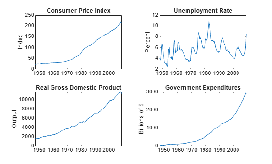
figure
plot(DataTimeTable.Time,DataTimeTable.CPIAUCSL);
title("Consumer Price Index")
ylabel("Index")
xlabel("Date")

Figure contains an axes object. The axes object with title Consumer Price Index, xlabel Date, ylabel Index contains an object of type line.

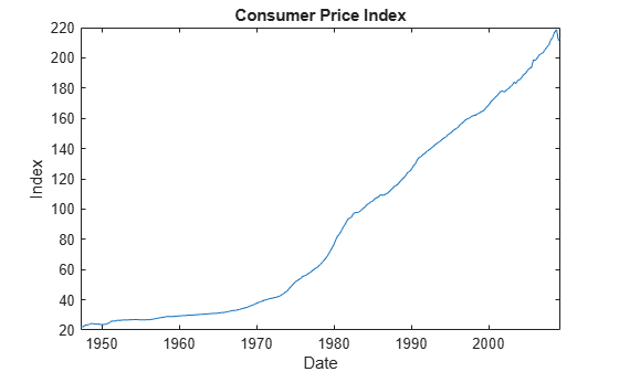
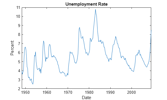
figure
plot(DataTimeTable.Time,DataTimeTable.UNRATE);
title("Unemployment Rate")
ylabel("Percent")
xlabel("Date")

Figure contains an axes object. The axes object with title Unemployment Rate, xlabel Date, ylabel Percent contains an object of type line.

Stabilize the CPI by converting it to a series of growth rates. Synchronize the two series by removing the first observation from the unemployment rate series. Create a new data set containing the transformed variables, and do not include any rows containing at least one missing observation.

rcpi = price2ret(DataTimeTable.CPIAUCSL);
unrate = DataTimeTable.UNRATE(2:end);
dates = DataTimeTable.Time(2:end);
Data = array2timetable([rcpi unrate],RowTimes=dates, ...
    VariableNames=["RCPI" "UNRATE"]);
Data = rmmissing(Data);

Create a default VAR(4) model by using the shorthand syntax.

Mdl = varm(2,4);
Mdl.SeriesNames = Data.Properties.VariableNames;

Estimate the model using the entire data set.

EstMdl = estimate(Mdl,Data.Variables);

EstMdl is a fully specified, estimated varm model object.

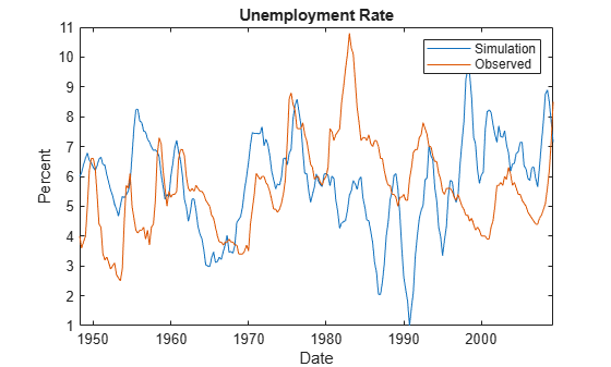
Simulate a response series path from the estimated model with length equal to the path in the data.

rng(1); % For reproducibility
numobs = height(Data);
Y = simulate(EstMdl,numobs);

Y is a 245-by-2 matrix of simulated responses. The first and second columns contain the simulated CPI growth rate and unemployment rate, respectively.

Plot the simulated and true responses.

figure
plot(Data.Time,Y(:,1));
hold on
plot(Data.Time,Data.RCPI)
title("CPI Growth Rate");
ylabel("Growth Rate")
xlabel("Date")
legend("Simulation","Observed")
hold off

Figure contains an axes object. The axes object with title CPI Growth Rate, xlabel Date, ylabel Growth Rate contains 2 objects of type line. These objects represent Simulation, Observed.

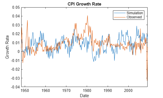
figure
plot(Data.Time,Y(:,2));
hold on
plot(Data.Time,Data.UNRATE)
ylabel("Percent")
xlabel("Date")
title("Unemployment Rate")
legend("Simulation","Observed")
hold off

Figure contains an axes object. The axes object with title Unemployment Rate, xlabel Date, ylabel Percent contains 2 objects of type line. These objects represent Simulation, Observed.

Illustrate the relationship between simulate and filter by estimating a 4-D VAR(2) model of the four response series in Johansen's Danish data set. Simulate a single path of responses using the fitted model and the historical data as initial values, and then filter a random set of Gaussian disturbances through the estimated model using the same presample responses.

Load Johansen's Danish economic data.

load Data_JDanish

For details on the variables, enter Description.

Create a default 4-D VAR(2) model.

Mdl = varm(4,2);
Mdl.SeriesNames = DataTimeTable.Properties.VariableNames;

Estimate the VAR(2) model using the entire data set.

EstMdl = estimate(Mdl,DataTimeTable.Variables);

When reproducing the results of simulate and filter:

  • Set the same random number seed using rng.

  • Specify the same presample response data using the Y0 name-value argument.

Set the default random seed. Simulate 100 observations by passing the estimated model to simulate. Specify the entire data set as the presample.

rng("default")
YSim = simulate(EstMdl,100,Y0=DataTimeTable.Variables);

YSim is a 100-by-4 matrix of simulated responses. Columns correspond to the columns of the variables in Data.

Set the default random seed. Simulate 4 series of 100 observations from the standard Gaussian distribution.

rng("default")
Z = randn(100,4);

Filter the Gaussian values through the estimated model. Specify the entire data set as the presample.

YFilter = filter(EstMdl,Z,Y0=DataTimeTable.Variables);

YFilter is a 100-by-4 matrix of simulated responses. Columns correspond to the columns of the variables in the data Data. Before filtering the disturbances, filter scales Z by the lower triangular Cholesky factor of the model covariance in EstMdl.Covariance.

Compare the resulting responses between filter and simulate.

(YSim - YFilter)'*(YSim - YFilter)
ans = 4×4

     0     0     0     0
     0     0     0     0
     0     0     0     0
     0     0     0     0

The results are identical.

Load Johansen's Danish economic data. Remove all missing observations.

load Data_JDanish
Data = rmmissing(Data);
T = height(Data);

For details on the variables, enter Description.

Create a default 4-D VAR(2) model.

Mdl = varm(4,2);

Estimate the VAR(2) model using the entire data set.

EstMdl = estimate(Mdl,Data);

When reproducing the results of simulate and filter:

  • Set the same random number seed using rng.

  • Specify the same presample response data using the Y0 name-value argument.

Simulate 100 paths of T – EstMdl.P, the effective sample size, responses, and corresponding innovations by passing the estimated model to simulate. Specify the same matrix of presample as the presample used in estimation (the earliest Mdl.P observations, by default).

rng("default")
p = Mdl.P;
numobs = T - p;
PS = Data(1:p,:);
[YSim,ESim] = simulate(EstMdl,numobs,NumPaths=100,Y0=PS);
size(YSim)
ans = 1×3

    53     4   100

YSim and ESim are 53-by-4-by-1000 numeric arrays of simulated responses and innovations, respectively. Each row corresponds to a period in the simulation horizon, each column corresponds to the variable in EstMdl.SeriesNames, and pages are separate, independently simulated paths.

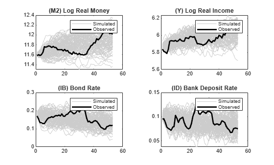
Plot each simulated response and innovations variable with their observations.

figure
InSample = Data((p+1):end,:);
tiledlayout(2,2)
for j = 1:numel(EstMdl.SeriesNames)
    nexttile
    h1 = plot(squeeze(YSim(:,j,:)),Color=[0.8 0.8 0.8]);
    hold on
    h2 = plot(InSample(:,j),Color="k",LineWidth=2);
    hold off
    title(series(j))
    legend([h1(1) h2],["Simulated" "Observed"])
end

Figure contains 4 axes objects. Axes object 1 with title (M2) Log Real Money contains 101 objects of type line. These objects represent Simulated, Observed. Axes object 2 with title (Y) Log Real Income contains 101 objects of type line. These objects represent Simulated, Observed. Axes object 3 with title (IB) Bond Rate contains 101 objects of type line. These objects represent Simulated, Observed. Axes object 4 with title (ID) Bank Deposit Rate contains 101 objects of type line. These objects represent Simulated, Observed.

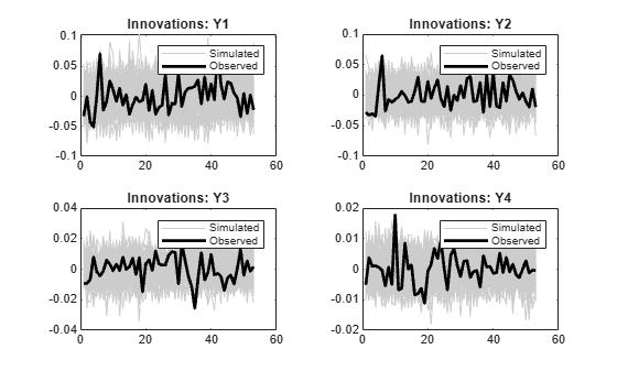
E = infer(EstMdl,InSample,Y0=PS);
figure
tiledlayout(2,2)
for j = 1:numel(EstMdl.SeriesNames)
    nexttile
    h1 = plot(squeeze(ESim(:,j,:)),Color=[0.8 0.8 0.8]);
    hold on
    h2 = plot(E(:,j),Color="k",LineWidth=2);
    hold off
    title("Innovations: " + EstMdl.SeriesNames{j})
    legend([h1(1) h2],["Simulated" "Observed"])
end

Figure contains 4 axes objects. Axes object 1 with title Innovations: Y1 contains 101 objects of type line. These objects represent Simulated, Observed. Axes object 2 with title Innovations: Y2 contains 101 objects of type line. These objects represent Simulated, Observed. Axes object 3 with title Innovations: Y3 contains 101 objects of type line. These objects represent Simulated, Observed. Axes object 4 with title Innovations: Y4 contains 101 objects of type line. These objects represent Simulated, Observed.

Since R2022b

Fit a VAR(4) model to the consumer price index (CPI) and unemployment rate data. Then, perform an unconditional simulation of the estimated model and return the simulated responses and corresponding innovations in a timetable. This example is based on Return Response Series in Matrix from Unconditional Simulation.

Load and Preprocess Data

Load the Data_USEconModel data set. Compute the CPI growth rate. Because the growth rate calculation consumes the earliest observation, include the rate variable in the timetable by prepending the series with NaN.

load Data_USEconModel
DataTimeTable.RCPI = [NaN; price2ret(DataTimeTable.CPIAUCSL)];
T = height(DataTimeTable)
T = 249

Prepare Timetable for Estimation

When you plan to supply a timetable directly to estimate, you must ensure it has all the following characteristics:

  • All selected response variables are numeric and do not contain any missing values.

  • The timestamps in the Time variable are regular, and they are ascending or descending.

Remove all missing values from the table, relative to the CPI rate (RCPI) and unemployment rate (UNRATE) series.

varnames = ["RCPI" "UNRATE"];
DTT = rmmissing(DataTimeTable,DataVariables=varnames);
T = height(DTT)
T = 245

rmmissing removes the four initial missing observations from the DataTimeTable to create a sub-table DTT. The variables RCPI and UNRATE of DTT do not have any missing observations.

Determine whether the sampling timestamps have a regular frequency and are sorted.

areTimestampsRegular = isregular(DTT,"quarters")
areTimestampsRegular = logical
   0

areTimestampsSorted = issorted(DTT.Time)
areTimestampsSorted = logical
   1

areTimestampsRegular = 0 indicates that the timestamps of DTT are irregular. areTimestampsSorted = 1 indicates that the timestamps are sorted. Macroeconomic series in this example are timestamped at the end of the month. This quality induces an irregularly measured series.

Remedy the time irregularity by shifting all dates to the first day of the quarter.

dt = DTT.Time;
dt = dateshift(dt,"start","quarter");
DTT.Time = dt;
areTimestampsRegular = isregular(DTT,"quarters")
areTimestampsRegular = logical
   1

DTT is regular with respect to time.

Create Model Template for Estimation

Create a default VAR(4) model by using the shorthand syntax. Specify the response variable names.

Mdl = varm(2,4);
Mdl.SeriesNames = varnames;

Fit Model to Data

Estimate the model. Pass the entire timetable DTT. By default, estimate selects the response variables in Mdl.SeriesNames to fit to the model. Alternatively, you can use the ResponseVariables name-value argument.

EstMdl = estimate(Mdl,DTT);
p = EstMdl.P
p = 4

Perform Unconditional Simulation of Estimated Model

Simulate a response and innovations path from the estimated model and return the simulated series as variables in a timetable. simulate requires information for the output timetable, such as variable names, sampling times for the simulation horizon, and sampling frequency. Therefore, supply a presample of the earliest p = 4 observations of the data DTT, from which simulate infers the required timetable information. Specify a simulation horizon of numobs – p.

rng(1) % For reproducibility
PSTbl = DTT(1:p,:);
numobs = T - p;
Tbl = simulate(EstMdl,T,Presample=PSTbl);
size(Tbl)
ans = 1×2

   245     4

PSTbl
PSTbl=4×15 timetable
    Time      COE     CPIAUCSL    FEDFUNDS    GCE      GDP     GDPDEF    GPDI    GS10    HOANBS    M1SL    M2SL    PCEC     TB3MS    UNRATE      RCPI   
    _____    _____    ________    ________    ____    _____    ______    ____    ____    ______    ____    ____    _____    _____    ______    _________

    Q1-48    137.9      23.5        NaN       37.6    260.4    16.111      45    NaN     55.036    NaN     NaN     170.5       1        4      0.0038371
    Q2-48    139.6     24.15        NaN       39.7    267.3    16.254    48.1    NaN     55.007    NaN     NaN     174.3       1      3.6       0.027284
    Q3-48    144.5     24.36        NaN       41.4    273.9    16.556    50.2    NaN     55.398    NaN     NaN     177.2    1.09      3.8      0.0086581
    Q4-48    145.9     24.05        NaN       43.5    275.2    16.597    49.1    NaN     54.885    NaN     NaN     178.1    1.16        4      -0.012807

head(Tbl)
    Time     RCPI_Responses    UNRATE_Responses    RCPI_Innovations    UNRATE_Innovations
    _____    ______________    ________________    ________________    __________________

    Q1-49       0.0037294           4.6036            -0.0038547             0.25039     
    Q2-49       0.0064827           5.0083             0.0070154            0.027504     
    Q3-49      -0.0073358           5.4981            -0.0045047             0.25199     
    Q4-49      -0.0057328           5.7007            -0.0065904             0.10593     
    Q1-50      -0.0060454           5.8687             -0.005022             0.13824     
    Q2-50      -0.0084475           5.5758            -0.0034013            -0.26192     
    Q3-50      -0.0067066           5.4129            -0.0033182             0.13055     
    Q4-50      -0.0020759           5.2191             0.0010595             0.11135     

Tbl is a 241-by-4 matrix of simulated responses and innovations. RCPI_Responses is the simulated path of the CPI growth rate and RCPI_Innovations is the corresponding innovations series, and the variables associated with the unemployment rate are similar. The timestamps of Tbl follow directly from the timestamps of PSTbl, and they have the same sampling frequency.

Since R2022b

Estimate a VAR(4) model of the consumer price index (CPI), the unemployment rate, and the gross domestic product (GDP). Include a linear regression component containing the current and the last four quarters of government consumption expenditures and investment. Simulate multiple paths from the estimated model.

Load the Data_USEconModel data set. Compute the real GDP.

load Data_USEconModel
DataTimeTable.RGDP = DataTimeTable.GDP./DataTimeTable.GDPDEF*100;

Plot all variables on separate plots.

figure
tiledlayout(2,2)
nexttile
plot(DataTimeTable.Time,DataTimeTable.CPIAUCSL);
ylabel("Index")
title("Consumer Price Index")
nexttile
plot(DataTimeTable.Time,DataTimeTable.UNRATE);
ylabel("Percent")
title("Unemployment Rate")
nexttile
plot(DataTimeTable.Time,DataTimeTable.RGDP);
ylabel("Output")
title("Real Gross Domestic Product")
nexttile
plot(DataTimeTable.Time,DataTimeTable.GCE);
ylabel("Billions of $")
title("Government Expenditures")

Figure contains 4 axes objects. Axes object 1 with title Consumer Price Index, ylabel Index contains an object of type line. Axes object 2 with title Unemployment Rate, ylabel Percent contains an object of type line. Axes object 3 with title Real Gross Domestic Product, ylabel Output contains an object of type line. Axes object 4 with title Government Expenditures, ylabel Billions of $ contains an object of type line.

Stabilize the CPI, GDP, and GCE by converting each to a series of growth rates. Synchronize the unemployment rate series with the others by removing its first observation.

varnames = ["CPIAUCSL" "RGDP" "GCE"];
DTT = varfun(@price2ret,DataTimeTable,InputVariables=varnames);
DTT.Properties.VariableNames = varnames;
DTT.UNRATE = DataTimeTable.UNRATE(2:end);

Make the time base regular.

dt = DTT.Time;
dt = dateshift(dt,"start","quarter");
DTT.Time = dt;

Expand the GCE rate series to a matrix that includes the first lagged series through the fourth lag series.

RGCELags = lagmatrix(DTT,1:4,DataVariables="GCE");
DTT = [DTT RGCELags];
DTT = rmmissing(DTT);

Create separate presample and estimation sample data sets. The presample contains the earliest p = 4 observations, and the estimation sample contains the rest of the data.

p = 4;
PS = DTT(1:p,:);
InSample = DTT((p+1):end,:);
respnames = ["CPIAUCSL" "UNRATE" "RGDP"];
idx = endsWith(InSample.Properties.VariableNames,"GCE");
prednames = InSample.Properties.VariableNames(idx);

Create a default VAR(4) model by using the shorthand syntax. Specify the response variable names.

Mdl = varm(3,p);
Mdl.SeriesNames = respnames;

Estimate the model using the entire sample. Specify the GCE and its lags as exogenous predictor data for the regression component.

EstMdl = estimate(Mdl,InSample,Presample=PS,PredictorVariables=prednames);

Generate 100 random response and innovations paths from the estimated model by performing an unconditional simulation. Specify that the length of the paths is the same as the length of the estimation sample period. Supply the presample and estimation sample data.

rng(1) % For reproducibility
numpaths = 100;
numobs = height(InSample);
Tbl = simulate(EstMdl,numobs,NumPaths=numpaths, ...
    Presample=PS,InSample=InSample,PredictorVariables=prednames);
size(Tbl)
ans = 1×2

   240    14

head(Tbl)
    Time      CPIAUCSL        RGDP          GCE        UNRATE     Lag1GCE       Lag2GCE       Lag3GCE       Lag4GCE      CPIAUCSL_Responses    UNRATE_Responses    RGDP_Responses    CPIAUCSL_Innovations    UNRATE_Innovations    RGDP_Innovations
    _____    __________    __________    __________    ______    __________    __________    __________    __________    __________________    ________________    ______________    ____________________    __________________    ________________

    Q1-49    0.00041815    -0.0031645      0.036603     6.2        0.047147       0.04948       0.04193      0.054347       1x100 double         1x100 double       1x100 double         1x100 double           1x100 double         1x100 double  
    Q2-49    -0.0071324      0.011385    -0.0021164     6.6        0.036603      0.047147       0.04948       0.04193       1x100 double         1x100 double       1x100 double         1x100 double           1x100 double         1x100 double  
    Q3-49    -0.0059122     -0.010366     -0.012793     6.6      -0.0021164      0.036603      0.047147       0.04948       1x100 double         1x100 double       1x100 double         1x100 double           1x100 double         1x100 double  
    Q4-49     0.0012698      0.040091     -0.021693     6.3       -0.012793    -0.0021164      0.036603      0.047147       1x100 double         1x100 double       1x100 double         1x100 double           1x100 double         1x100 double  
    Q1-50      0.010101      0.029649      0.010905     5.4       -0.021693     -0.012793    -0.0021164      0.036603       1x100 double         1x100 double       1x100 double         1x100 double           1x100 double         1x100 double  
    Q2-50       0.01908       0.03844    -0.0043478     4.4        0.010905     -0.021693     -0.012793    -0.0021164       1x100 double         1x100 double       1x100 double         1x100 double           1x100 double         1x100 double  
    Q3-50      0.025954      0.017994      0.075508     4.3      -0.0043478      0.010905     -0.021693     -0.012793       1x100 double         1x100 double       1x100 double         1x100 double           1x100 double         1x100 double  
    Q4-50      0.035395       0.01197       0.14807     3.4        0.075508    -0.0043478      0.010905     -0.021693       1x100 double         1x100 double       1x100 double         1x100 double           1x100 double         1x100 double  

Tbl is a 240-by-14 timetable of estimation sample data, simulated responses (denoted responseName_Responses), and corresponding innovations (denoted responseName_Innovations). The simulated response and innovations variables are 240-by-100 matrices, where each row is a period in the estimation sample and each column is a separate, independently generated path.

For each time in the estimation sample, compute the mean vector of the simulated responses among all paths.

idx = endsWith(Tbl.Properties.VariableNames,"_Responses");
simrespnames = Tbl.Properties.VariableNames(idx);
MeanSim = varfun(@(x)mean(x,2),Tbl,InputVariables=simrespnames);

MeanSim is a 240-by-3 timetable containing the average of the simulated responses at each time point.

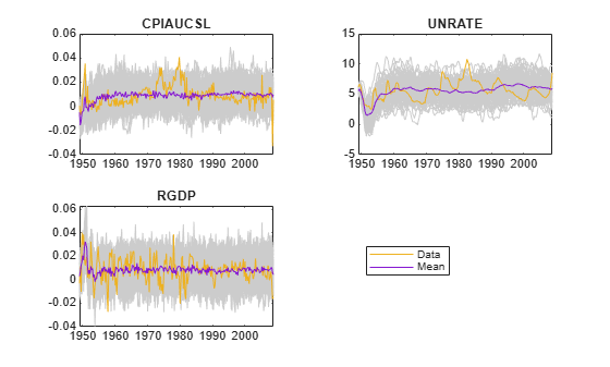
Plot the simulated responses, their averages, and the data.

figure
tiledlayout(2,2)
for j = 1:Mdl.NumSeries
    nexttile
    plot(Tbl.Time,Tbl{:,simrespnames(j)},Color=[0.8,0.8,0.8])
    title(Mdl.SeriesNames{j});
    hold on
    h1 = plot(Tbl.Time,Tbl{:,respnames(j)});
    h2 = plot(Tbl.Time,MeanSim{:,"Fun_"+simrespnames(j)});
    hold off
end

hl = legend([h1 h2],"Data","Mean");
hl.Position = [0.6 0.25 hl.Position(3:4)];

Figure contains 3 axes objects. Axes object 1 with title CPIAUCSL contains 102 objects of type line. Axes object 2 with title UNRATE contains 102 objects of type line. Axes object 3 with title RGDP contains 102 objects of type line. These objects represent Data, Mean.

Since R2022b

Perform a conditional simulation of the VAR model in Return Timetable of Responses and Innovations from Unconditional Simulation, in which economists hypothesize that the unemployment rate is 6% for 15 quarters after the end of the sampling period (from Q2 of 2009 through Q4 of 2012).

Load and Preprocess Data

Load the Data_USEconModel data set. Compute the CPI growth rate. Because the growth rate calculation consumes the earliest observation, include the rate variable in the timetable by prepending the series with NaN.

load Data_USEconModel
DataTimeTable.RCPI = [NaN; price2ret(DataTimeTable.CPIAUCSL)];

Prepare Timetable for Estimation

Remove all missing values from the table, relative to the CPI rate (RCPI) and unemployment rate (UNRATE) series.

varnames = ["RCPI" "UNRATE"];
DTT = rmmissing(DataTimeTable,DataVariables=varnames);

Remedy the time irregularity by shifting all dates to the first day of the quarter.

dt = DTT.Time;
dt = dateshift(dt,"start","quarter");
DTT.Time = dt;

Create Model Template for Estimation

Create a default VAR(4) model by using the shorthand syntax. Specify the response variable names.

p = 4;
Mdl = varm(2,p);
Mdl.SeriesNames = varnames;

Fit Model to Data

Estimate the model. Pass the entire timetable DTT. By default, estimate selects the response variables in Mdl.SeriesNames to fit to the model. Alternatively, you can use the ResponseVariables name-value argument.

EstMdl = estimate(Mdl,DTT);

Prepare for Conditional Simulation of Estimated Model

Suppose economists hypothesize that the unemployment rate will be at 6% for the next 15 quarters.

Create a timetable with the following qualities:

  • The timestamps are regular with respect to the estimation sample timestamps and they are ordered from Q2 of 2009 through Q4 of 2012.

  • The variable RCPI (and, consequently, all other variables in DTT) is a 15-by-1 vector of NaN values.

  • The variable UNRATE is a 15-by-1 vector, where each element is 6.

numobs = 15;
shdt = DTT.Time(end) + calquarters(1:numobs);
DTTCondSim = retime(DTT,shdt,"fillwithmissing");
DTTCondSim.UNRATE = ones(numobs,1)*6;

DTTCondSim is a 15-by-15 timetable that follows directly, in time, from DTT, and both timetables have the same variables. All variables in DTTCondSim contain NaN values, except for UNRATE, which is a vector composed of the value 6.

Perform Conditional Simulation of Estimated Model

Simulate the CPI growth rate given the hypothesis by supplying the conditioning data DTTCondSim and specifying the response variable names. Generate 1000 paths. Because the simulation horizon is beyond the estimation sample data, supply the estimation sample as a presample to initialize the model.

rng(1) % For reproducibility
Tbl = simulate(EstMdl,numobs,NumPaths=1000, ...
    InSample=DTTCondSim,ResponseVariables=EstMdl.SeriesNames, ...
    Presample=DTT,PresampleResponseVariables=EstMdl.SeriesNames);
size(Tbl)
ans = 1×2

    15    19

idx = endsWith(Tbl.Properties.VariableNames,["_Responses" "_Innovations"]);
head(Tbl(:,idx))
    Time     RCPI_Responses    UNRATE_Responses    RCPI_Innovations    UNRATE_Innovations
    _____    ______________    ________________    ________________    __________________

    Q2-09    1x1000 double      1x1000 double       1x1000 double        1x1000 double   
    Q3-09    1x1000 double      1x1000 double       1x1000 double        1x1000 double   
    Q4-09    1x1000 double      1x1000 double       1x1000 double        1x1000 double   
    Q1-10    1x1000 double      1x1000 double       1x1000 double        1x1000 double   
    Q2-10    1x1000 double      1x1000 double       1x1000 double        1x1000 double   
    Q3-10    1x1000 double      1x1000 double       1x1000 double        1x1000 double   
    Q4-10    1x1000 double      1x1000 double       1x1000 double        1x1000 double   
    Q1-11    1x1000 double      1x1000 double       1x1000 double        1x1000 double   

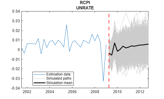
Tbl is a 15-by-19 matrix of simulated responses and innovations of RCPI given UNRATE is 6% for the next 15 quarters. RCPI_Responses contains the simulated paths of the CPI growth rate and RCPI_Innovations contains the corresponding innovations series. UNRATE_Responses is a 15-by-1000 matrix composed of the value 6. All other variables in Tbl are the variables and their values in DTTCondSim.

Plot the simulated values of the CPI growth rate and their mean with the final few values of the estimation sample data.

MeanRCPISim = mean(Tbl.RCPI_Responses,2);

figure
h1 = plot(DTT.Time((end-30):end),DTT.RCPI((end-30):end));
hold on
h2 = plot(Tbl.Time,Tbl.RCPI_Responses,Color=[0.8 0.8 0.8]);
h3 = plot(Tbl.Time,MeanRCPISim,Color="k",LineWidth=2);
xline(Tbl.Time(1),"r--",LineWidth=2)
hold off
title(EstMdl.SeriesNames)
legend([h1 h2(1) h3],["Estimation data" "Simulated paths" "Simulation mean"], ...
    Location="best")

Figure contains an axes object. The axes object with title RCPI UNRATE contains 1003 objects of type line, constantline. These objects represent Estimation data, Simulated paths, Simulation mean.

Input Arguments

collapse all

VAR model, specified as a varm model object created by varm or estimate. Mdl must be fully specified.

Number of random observations to generate per output path, specified as a positive integer. The output arguments Y and E, or Tbl, have numobs rows.

Data Types: double

Since R2022b

Presample data that provides initial values for the model Mdl, specified as a table or timetable with numprevars variables and numpreobs rows. The following situations describe when to use Presample:

  • Presample is required when simulate performs an unconditional simulation, which occurs under one of the following conditions:

    • You do not supply data in the simulation horizon (that is, you do not use the InSample name-value argument).

    • You specify only predictor data for the model regression component in the simulation horizon using the InSample and PredictorVariables name-value arguments, but you do not select any response variables from InSample.

  • Presample is optional when simulate performs a conditional simulation, that is, when you supply response data in the simulation horizon, on which to condition the simulated responses, by using the InSample and ResponseVariables name-value arguments. By default, simulate sets any necessary presample observations.

    • For stationary VAR processes without regression components, simulate sets presample observations to the unconditional mean μ=Φ1(L)c.

    • For nonstationary processes or models that contain a regression component, simulate sets presample observations to zero.

Regardless of the situation, simulate returns the simulated variables in the output table or timetable Tbl, which is commensurate with Presample.

Each row is a presample observation, and measurements in each row, among all paths, occur simultaneously. numpreobs must be at least Mdl.P. If you supply more rows than necessary, simulate uses the latest Mdl.P observations only.

Each variable is a numpreobs-by-numprepaths numeric matrix. Variables are associated with response series in Mdl.SeriesNames. To control presample variable selection, see the optional PresampleResponseVariables name-value argument.

For each variable, columns are separate, independent paths.

  • If variables are vectors, simulate applies them to each respective path to initialize the model for the simulation. Therefore, all respective response paths derive from common initial conditions.

  • Otherwise, for each variable ResponseK and each path j, simulate applies Presample.ResponseK(:,j) to produce Tbl.ResponseK(:,j). Variables must have at least numpaths columns, and simulate uses only the first numpaths columns.

If Presample is a timetable, all the following conditions must be true:

  • Presample must represent a sample with a regular datetime time step (see isregular).

  • The inputs InSample and Presample must be consistent in time such that Presample immediately precedes InSample with respect to the sampling frequency and order.

  • The datetime vector of sample timestamps Presample.Time must be ascending or descending.

If Presample is a table, the last row contains the latest presample observation.

Since R2022b

Future time series response or predictor data, specified as a table or timetable. InSample contains numvars variables, including numseries response variables yt or numpreds predictor variables xt for the model regression component. You can specify InSample only when other data inputs are tables or timetables.

Use InSample in the following situations:

  • Perform conditional simulation. You must also supply the response variable names in InSample by using the ResponseVariables name-value argument.

  • Supply future predictor data for either unconditional or conditional simulation. To supply predictor data, you must specify predictor variable names in InSample by using the PredictorVariables name-value argument. Otherwise, simulate ignores the model regression component.

simulate returns the simulated variables in the output table or timetable Tbl, which is commensurate with InSample.

Each row corresponds to an observation in the simulation horizon, the first row is the earliest observation, and measurements in each row, among all paths, occur simultaneously. InSample must have at least numobs rows to cover the simulation horizon. If you supply more rows than necessary, simulate uses only the first numobs rows.

Each response variable is a numeric matrix with numpaths columns. For each response variable K, columns are separate, independent paths. Specifically, path j of response variable ResponseK captures the state, or knowledge, of ResponseK as it evolves from the presample past (for example, Presample.ResponseK) into the future. For each selected response variable ResponseK:

  • If InSample.ResponseK is a vector, simulate applies to each of the numpaths output paths (see NumPaths).

  • Otherwise, InSample.ResponseK must have at least numpaths columns. If you supply more pages than necessary, simulate uses only the first numpaths columns.

Each predictor variable is a numeric vector. All predictor variables are present in the regression component of each response equation and apply to all response paths.

If InSample is a timetable, the following conditions apply:

  • InSample must represent a sample with a regular datetime time step (see isregular).

  • The datetime vector InSample.Time must be ascending or descending.

  • Presample must immediately precede InSample, with respect to the sampling frequency.

If InSample is a table, the last row contains the latest observation.

Elements of the response variables of InSample can be numeric scalars or missing values (indicated by NaN values). simulate treats numeric scalars as deterministic future responses that are known in advance, for example, set by policy. simulate simulates responses for corresponding NaN values conditional on the known values. Elements of selected predictor variables must be numeric scalars.

By default, simulate performs an unconditional simulation without a regression component in the model (each selected response variable is a numobs-by-numpaths matrix composed of NaN values indicating a complete lack of knowledge of the future state of all simulated responses). Therefore, variables in Tbl result from a conventional, unconditional Monte Carlo simulation.

For more details, see Algorithms.

Example: Consider simulating one path from a model composed of two response series, GDP and CPI, three periods into the future. Suppose that you have prior knowledge about some of the future values of the responses, and you want to simulate the unknown responses conditional on your knowledge. Specify InSample as a table containing the values that you know, and use NaN for values you do not know but want to simulate. For example, InSample=array2table([2 NaN; 0.1 NaN; NaN NaN],VariableNames=["GDP" "CPI"]) specifies that you have no knowledge of the future values of CPI, but you know that GDP is 2, 0.1, and unknown in periods 1, 2, and 3, respectively, in the simulation horizon.

Since R2022b

Variables to select from InSample to treat as response variables yt, specified as one of the following data types:

  • String vector or cell vector of character vectors containing numseries variable names in InSample.Properties.VariableNames

  • A length numseries vector of unique indices (integers) of variables to select from InSample.Properties.VariableNames

  • A length numvars logical vector, where ResponseVariables(j) = true selects variable j from InSample.Properties.VariableNames, and sum(ResponseVariables) is numseries

To perform conditional simulation, you must specify ResponseVariables to select the response variables in InSample for the conditioning data. ResponseVariables applies only when you specify InSample.

The selected variables must be numeric vectors (single path) or matrices (columns represent multiple independent paths) of the same width.

Example: ResponseVariables=["GDP" "CPI"]

Example: ResponseVariables=[true false true false] or ResponseVariable=[1 3] selects the first and third table variables as the response variables.

Data Types: double | logical | char | cell | string

Name-Value Arguments

Specify optional pairs of arguments as Name1=Value1,...,NameN=ValueN, where Name is the argument name and Value is the corresponding value. Name-value arguments must appear after other arguments, but the order of the pairs does not matter.

Before R2021a, use commas to separate each name and value, and enclose Name in quotes.

Example: simulate(Mdl,100,NumPaths=1000,Y0=PS) returns a numeric array of 1000, 100-period simulated response paths from Mdl and specifies the numeric array of presample response data PS.

Number of sample paths to generate, specified as a positive integer. The outputs Y and E have NumPaths pages, and each simulated response and innovation variable in the output Tbl is a numobs-by-NumPaths matrix.

Example: NumPaths=1000

Data Types: double

Presample responses that provide initial values for the model Mdl, specified as a numpreobs-by-numseries numeric matrix or a numpreobs-by-numseries-by-numprepaths numeric array. Use Y0 only when you supply optional data inputs as numeric arrays.

numpreobs is the number of presample observations. numprepaths is the number of presample response paths.

Each row is a presample observation, and measurements in each row, among all pages, occur simultaneously. The last row contains the latest presample observation. Y0 must have at least Mdl.P rows. If you supply more rows than necessary, simulate uses the latest Mdl.P observations only.

Each column corresponds to the response series name in Mdl.SeriesNames.

Pages correspond to separate, independent paths.

  • If Y0 is a matrix, simulate applies it to simulate each sample path (page). Therefore, all paths in the output argument Y derive from common initial conditions.

  • Otherwise, simulate applies Y0(:,:,j) to initialize simulating path j. Y0 must have at least numpaths pages, and simulate uses only the first numpaths pages.

By default, simulate sets any necessary presample observations.

  • For stationary VAR processes without regression components, simulate sets presample observations to the unconditional mean μ=Φ1(L)c.

  • For nonstationary processes or models that contain a regression component, simulate sets presample observations to zero.

Data Types: double

Since R2022b

Variables to select from Presample to use for presample data, specified as one of the following data types:

  • String vector or cell vector of character vectors containing numseries variable names in Presample.Properties.VariableNames

  • A length numseries vector of unique indices (integers) of variables to select from Presample.Properties.VariableNames

  • A length numprevars logical vector, where PresampleResponseVariables(j) = true selects variable j from Presample.Properties.VariableNames, and sum(PresampleResponseVariables) is numseries

PresampleResponseVariables applies only when you specify Presample.

The selected variables must be numeric vectors and cannot contain missing values (NaN).

PresampleResponseNames does not need to contain the same names as in Mdl.SeriesNames; simulate uses the data in selected variable PresampleResponseVariables(j) as a presample for Mdl.SeriesNames(j).

If the number of variables in Presample matches Mdl.NumSeries, the default specifies all variables in Presample. If the number of variables in Presample exceeds Mdl.NumSeries, the default matches variables in Presample to names in Mdl.SeriesNames.

Example: PresampleResponseVariables=["GDP" "CPI"]

Example: PresampleResponseVariables=[true false true false] or PresampleResponseVariable=[1 3] selects the first and third table variables for presample data.

Data Types: double | logical | char | cell | string

Predictor data for the regression component in the model, specified as a numeric matrix containing numpreds columns. Use X only when you supply optional data inputs as numeric arrays.

numpreds is the number of predictor variables (size(Mdl.Beta,2)).

Each row corresponds to an observation, and measurements in each row occur simultaneously. The last row contains the latest observation. X must have at least numobs rows. If you supply more rows than necessary, simulate uses only the latest numobs observations. simulate does not use the regression component in the presample period.

Each column is an individual predictor variable. All predictor variables are present in the regression component of each response equation.

simulate applies X to each path (page); that is, X represents one path of observed predictors.

By default, simulate excludes the regression component, regardless of its presence in Mdl.

Data Types: double

Since R2022b

Variables to select from InSample to treat as exogenous predictor variables xt, specified as one of the following data types:

  • String vector or cell vector of character vectors containing numpreds variable names in InSample.Properties.VariableNames

  • A length numpreds vector of unique indices (integers) of variables to select from InSample.Properties.VariableNames

  • A length numvars logical vector, where PredictorVariables(j) = true selects variable j from InSample.Properties.VariableNames, and sum(PredictorVariables) is numpreds

Regardless, selected predictor variable j corresponds to the coefficients Mdl.Beta(:,j).

PredictorVariables applies only when you specify InSample.

The selected variables must be numeric vectors and cannot contain missing values (NaN).

By default, simulate excludes the regression component, regardless of its presence in Mdl.

Example: PredictorVariables=["M1SL" "TB3MS" "UNRATE"]

Example: PredictorVariables=[true false true false] or PredictorVariable=[1 3] selects the first and third table variables as the response variables.

Data Types: double | logical | char | cell | string

Future multivariate response series for conditional simulation, specified as a numeric matrix or array containing numseries columns. Use YF only when you supply optional data inputs as numeric arrays.

Each row corresponds to observations in the simulation horizon, and the first row is the earliest observation. Specifically, row j in sample path k (YF(j,:,k)) contains the responses j periods into the future. YF must have at least numobs rows to cover the simulation horizon. If you supply more rows than necessary, simulate uses only the first numobs rows.

Each column corresponds to the response variable name in Mdl.SeriesNames.

Each page corresponds to a separate sample path. Specifically, path k (YF(:,:,k)) captures the state, or knowledge, of the response series as they evolve from the presample past (Y0) into the future.

  • If YF is a matrix, simulate applies YF to each of the numpaths output paths (see NumPaths).

  • Otherwise, YF must have at least numpaths pages. If you supply more pages than necessary, simulate uses only the first numpaths pages.

Elements of YF can be numeric scalars or missing values (indicated by NaN values). simulate treats numeric scalars as deterministic future responses that are known in advance, for example, set by policy. simulate simulates responses for corresponding NaN values conditional on the known values.

By default, YF is an array composed of NaN values indicating a complete lack of knowledge of the future state of all simulated responses. Therefore, simulate obtains the output responses Y from a conventional, unconditional Monte Carlo simulation.

For more details, see Algorithms.

Example: Consider simulating one path from a model composed of four response series three periods into the future. Suppose that you have prior knowledge about some of the future values of the responses, and you want to simulate the unknown responses conditional on your knowledge. Specify YF as a matrix containing the values that you know, and use NaN for values you do not know but want to simulate. For example, YF=[NaN 2 5 NaN; NaN NaN 0.1 NaN; NaN NaN NaN NaN] specifies that you have no knowledge of the future values of the first and fourth response series; you know the value for period 1 in the second response series, but no other value; and you know the values for periods 1 and 2 in the third response series, but not the value for period 3.

Data Types: double

Note

  • NaN values in Y0 and X indicate missing values. simulate removes missing values from the data by list-wise deletion. If Y0 is a 3-D array, then simulate performs these steps:

    1. Horizontally concatenate pages to form a numpreobs-by-numpaths*numseries matrix.

    2. Remove any row that contains at least one NaN from the concatenated data.

    In the case of missing observations, the results obtained from multiple paths of Y0 can differ from the results obtained from each path individually.

    For conditional simulation (see YF), if X contains any missing values in the latest numobs observations, then simulate issues an error.

  • simulate issues an error when selected response variables from Presample and selected predictor variables from InSample contain any missing values.

Output Arguments

collapse all

Simulated multivariate response series, returned as a numobs-by-numseries numeric matrix or a numobs-by-numseries-by-numpaths numeric array. simulate returns Y only when you supply optional data sets as numeric matrices or arrays, for example, you use the Y0 name-value argument.

Y represents the continuation of the presample responses in Y0.

Each row is a time point in the simulation horizon. Values in a row, among all pages, occur simultaneously. The last row contains the latest simulated values.

Each column corresponds to the response series name in Mdl.SeriesNames.

Pages correspond to separate, independently simulated paths.

If you specify future responses for conditional simulation using the YF name-value argument, the known values in YF appear in the same positions in Y. However, Y contains simulated values for the missing observations in YF.

Simulated multivariate model innovations series, returned as a numobs-by-numseries numeric matrix or a numobs-by-numseries-by-numpaths numeric array. simulate returns E only when you supply optional data sets as numeric matrices or arrays, for example, you use the Y0 name-value argument.

Elements of E and Y correspond.

If you specify future responses for conditional simulation (see the YF name-value argument), simulate infers the innovations from the known values in YF and places the inferred innovations in the corresponding positions in E. For the missing observations in YF, simulate draws from the Gaussian distribution conditional on any known values, and places the draws in the corresponding positions in E.

Since R2022b

Simulated multivariate response, model innovations, and other variables, returned as a table or timetable, the same data type as Presample or InSample. simulate returns Tbl only when you supply at least one of the inputs Presample and InSample.

Tbl contains the following variables:

  • The simulated paths within the simulation horizon of the selected response series yt. Each simulated response variable in Tbl is a numobs-by-numpaths numeric matrix, where numobs is the value of NumObs and numpaths is the value of NumPaths. Each row corresponds to a time in the simulation horizon and each column corresponds to a separate path. simulate names the simulated response variable ResponseK ResponseK_Responses. For example, if Mdl.Series(K) is GDP, Tbl contains a variable for the corresponding simulated response with the name GDP_Responses. If you specify ResponseVariables, ResponseK is ResponseVariable(K). Otherwise, ResponseK is PresampleResponseVariable(K).

  • The simulated paths within the simulation horizon of the innovations εt corresponding to yt. Each simulated innovations variable in Tbl is a numobs-by-numpaths numeric matrix. Each row corresponds to a time in the simulation horizon and each column corresponds to a separate path. simulate names the simulated innovations variable of response ResponseK ResponseK_Innovations. For example, if Mdl.Series(K) is GDP, Tbl contains a variable for the corresponding innovations with the name GDP_Innovations.

If Tbl is a timetable, the following conditions hold:

  • The row order of Tbl, either ascending or descending, matches the row order of InSample, when you specify it. If you do not specify InSample and you specify Presample, the row order of Tbl is the same as the row order Presample.

  • If you specify InSample, row times Tbl.Time are InSample.Time(1:numobs). Otherwise, Tbl.Time(1) is the next time after Presample(end) relative to the sampling frequency, and Tbl.Time(2:numobs) are the following times relative to the sampling frequency.

Algorithms

Suppose Y0 and YF are the presample and future response data specified by the numeric data inputs in Y0 and YF or the selected variables from the input tables or timetables Presample and InSample. Similarly, suppose E contains the simulated model innovations as returned in the numeric array E or the table or timetable Tbl.

  • simulate performs conditional simulation using this process for all pages k = 1,...,numpaths and for each time t = 1,...,numobs.

    1. simulate infers (or inverse filters) the model innovations for all response variables (E(t,:,k) from the known future responses (YF(t,:,k)). In E, simulate mimics the pattern of NaN values that appears in YF.

    2. For the missing elements of E at time t, simulate performs these steps.

      1. Draw Z1, the random, standard Gaussian distribution disturbances conditional on the known elements of E.

      2. Scale Z1 by the lower triangular Cholesky factor of the conditional covariance matrix. That is, Z2 = L*Z1, where L = chol(C,"lower") and C is the covariance of the conditional Gaussian distribution.

      3. Impute Z2 in place of the corresponding missing values in E.

    3. For the missing values in YF, simulate filters the corresponding random innovations through the model Mdl.

  • simulate uses this process to determine the time origin t0 of models that include linear time trends.

    • If you do not specify Y0, then t0 = 0.

    • Otherwise, simulate sets t0 to size(Y0,1)Mdl.P. Therefore, the times in the trend component are t = t0 + 1, t0 + 2,..., t0 + numobs. This convention is consistent with the default behavior of model estimation in which estimate removes the first Mdl.P responses, reducing the effective sample size. Although simulate explicitly uses the first Mdl.P presample responses in Y0 to initialize the model, the total number of observations in Y0 (excluding any missing values) determines t0.

References

[1] Hamilton, James D. Time Series Analysis. Princeton, NJ: Princeton University Press, 1994.

[2] Johansen, S. Likelihood-Based Inference in Cointegrated Vector Autoregressive Models. Oxford: Oxford University Press, 1995.

[3] Juselius, K. The Cointegrated VAR Model. Oxford: Oxford University Press, 2006.

[4] Lütkepohl, H. New Introduction to Multiple Time Series Analysis. Berlin: Springer, 2005.

Version History

Introduced in R2017a

expand all