Main Content

infer

Infer vector autoregression model (VAR) innovations

Description

example

E = infer(Mdl,Y) returns a numeric array E containing the series of multivariate inferred innovations from evaluating the fully specified VAR(p) model Mdl at the numeric array of response data Y. For example, if Mdl is a VAR model fit to the response data Y, E contains the residuals.

example

Tbl2 = infer(Mdl,Tbl1) returns the table or timetable Tbl2 containing the multivariate residuals from evaluating the fully specified VAR(p) model Mdl at the response variables in the table or timetable of data Tbl1. (since R2022b)

infer selects the variables in Mdl.SeriesNames or all variables in Tbl1. To select different response variables in Tbl1 at which to evaluate the model, use the ResponseVariables name-value argument.

example

___ = infer(___,Name=Value) specifies options using one or more name-value arguments in addition to any of the input argument combinations in previous syntaxes. infer returns the output argument combination for the corresponding input arguments. For example, infer(Mdl,Y,Y0=PS,X=Exo) computes the residuals of the VAR(p) model Mdl at the matrix of response data Y, and specifies the matrix of presample response data PS and the matrix of exogenous predictor data Exo.

Supply all input data using the same data type. Specifically:

  • If you specify the numeric matrix Y, optional data sets must be numeric arrays and you must use the appropriate name-value argument. For example, to specify a presample, set the Y0 name-value argument to a numeric matrix of presample data.

  • If you specify the table or timetable Tbl1, optional data sets must be tables or timetables, respectively, and you must use the appropriate name-value argument. For example, to specify a presample, set the Presample name-value argument to a table or timetable of presample data.

example

[___,logL] = infer(___) returns the loglikelihood objective function value logL evaluated at the specified data.

Examples

collapse all

Fit a VAR(4) model to the consumer price index (CPI) and unemployment rate data in a matrix. Then, infer the model innovations (residuals) from the estimated model.

Load the Data_USEconModel data set.

load Data_USEconModel

Plot the two series on separate plots.

figure
plot(DataTimeTable.Time,DataTimeTable.CPIAUCSL)
title("Consumer Price Index")
ylabel("Index")
xlabel("Date")

Figure contains an axes object. The axes object with title Consumer Price Index, xlabel Date, ylabel Index contains an object of type line.

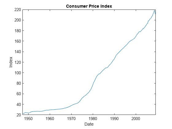
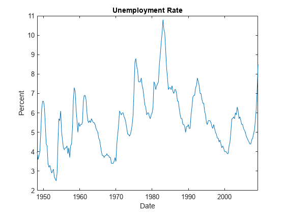
figure
plot(DataTimeTable.Time,DataTimeTable.UNRATE)
title("Unemployment Rate")
ylabel("Percent")
xlabel("Date")

Figure contains an axes object. The axes object with title Unemployment Rate, xlabel Date, ylabel Percent contains an object of type line.

Stabilize the CPI by converting it to a series of growth rates. Synchronize the two series by removing the first observation from the unemployment rate series.

rcpi = price2ret(DataTimeTable.CPIAUCSL);
unrate = DataTimeTable.UNRATE(2:end);

Create a default VAR(4) model by using the shorthand syntax.

Mdl = varm(2,4);

Estimate the model using the entire data set.

EstMdl = estimate(Mdl,[rcpi unrate]);

EstMdl is a fully specified, estimated varm model object.

Infer innovations from the estimated model. Supply the same response data that the model was fit to as a numeric matrix.

E = infer(EstMdl,[rcpi unrate]);

E is a 241-by-2 matrix of inferred innovations. The first and second columns contain the residuals corresponding to the CPI growth rate and unemployment rate, respectively.

Alternatively, you can return residuals when you call estimate by supplying an output variable in the fourth position.

Plot the residuals on separate plots. Synchronize the residuals with the dates by removing any missing observations from the data and removing the first Mdl.P dates.

idx = all(~isnan([rcpi unrate]),2);
datesr = DataTimeTable.Time(idx);

figure
plot(datesr((Mdl.P + 1):end),E(:,1));
ylabel("Consumer Price Index")
xlabel("Date")
title("Residual Plot")
hold on
yline(0,"r--");
hold off

Figure contains an axes object. The axes object with title Residual Plot, xlabel Date, ylabel Consumer Price Index contains 2 objects of type line, constantline.

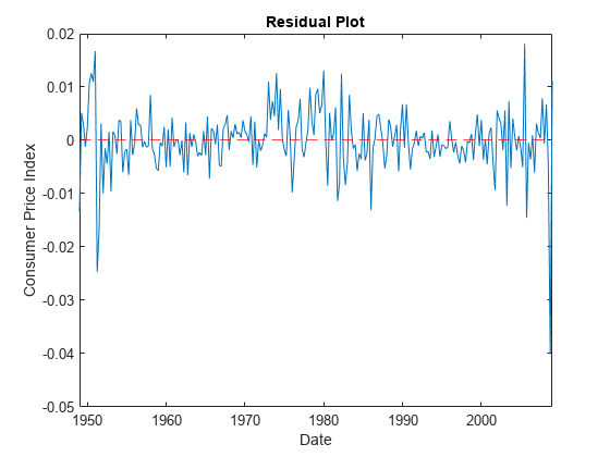
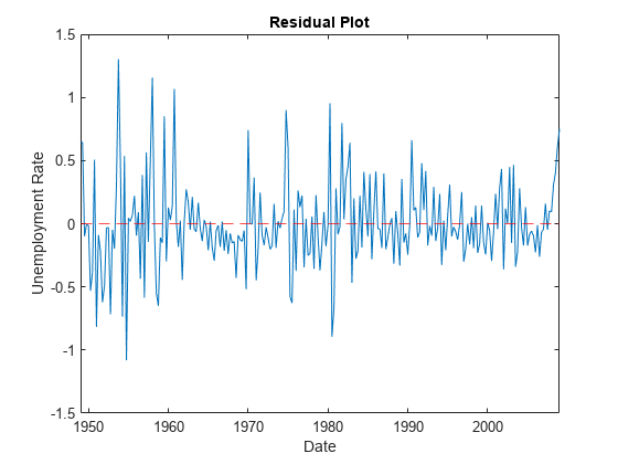
figure
plot(datesr((Mdl.P + 1):end),E(:,2))
ylabel("Unemployment Rate")
xlabel("Date")
title("Residual Plot")
hold on
yline(0,"r--");
hold off

Figure contains an axes object. The axes object with title Residual Plot, xlabel Date, ylabel Unemployment Rate contains 2 objects of type line, constantline.

The residuals corresponding to the CPI growth rate exhibit heteroscedasticity because the series appears to cycle through periods of higher and lower variance.

Since R2022b

Fit a VAR(4) model to the consumer price index (CPI) and unemployment rate data in a timetable. Then, infer the model innovations (residuals) from the estimated model.

Load and Preprocess Data

Load the Data_USEconModel data set. Compute the CPI growth rate. Because the growth rate calculation consumes the earliest observation, include the rate variable in the timetable by prepending the series with NaN.

load Data_USEconModel
DataTimeTable.RCPI = [NaN; price2ret(DataTimeTable.CPIAUCSL)];
numobs = height(DataTimeTable)
numobs = 249

Prepare Timetable for Estimation

When you plan to supply a timetable directly to estimate, you must ensure it has all the following characteristics:

  • All selected response variables are numeric and do not contain any missing values.

  • The timestamps in the Time variable are regular, and they are ascending or descending.

Remove all missing values from the table, relative to the CPI rate (RCPI) and unemployment rate (UNRATE) series.

varnames = ["RCPI" "UNRATE"];
DTT = rmmissing(DataTimeTable,DataVariables=varnames);
numobs = height(DTT)
numobs = 245

rmmissing removes the four initial missing observations from the DataTimeTable to create a sub-table DTT. The variables RCPI and UNRATE of DTT do not have any missing observations.

Determine whether the sampling timestamps have a regular frequency and are sorted.

areTimestampsRegular = isregular(DTT,"quarters")
areTimestampsRegular = logical
   0

areTimestampsSorted = issorted(DTT.Time)
areTimestampsSorted = logical
   1

areTimestampsRegular = 0 indicates that the timestamps of DTT are irregular. areTimestampsSorted = 1 indicates that the timestamps are sorted. Macroeconomic series in this example are timestamped at the end of the month. This quality induces an irregularly measured series.

Remedy the time irregularity by shifting all dates to the first day of the quarter.

dt = DTT.Time;
dt = dateshift(dt,"start","quarter");
DTT.Time = dt;
areTimestampsRegular = isregular(DTT,"quarters")
areTimestampsRegular = logical
   1

DTT is regular with respect to time.

Create Model Template for Estimation

Create a default VAR(4) model by using the shorthand syntax. Specify the response variable names.

Mdl = varm(2,4);
Mdl.SeriesNames = varnames;

Fit Model to Data

Estimate the model. Pass the entire timetable DTT. By default, estimate selects the response variables in Mdl.SeriesNames to fit to the model. Alternatively, you can use the ResponseVariables name-value argument.

EstMdl = estimate(Mdl,DTT);

Compute Residuals

Infer innovations from the estimated model. Supply the same response data that the model was fit to as a timetable. By default, infer selects the variables to use from EstMdl.SeriesNames.

Tbl = infer(EstMdl,DTT);
head(Tbl)
    Time      COE     CPIAUCSL    FEDFUNDS    GCE      GDP     GDPDEF    GPDI    GS10    HOANBS    M1SL    M2SL    PCEC     TB3MS    UNRATE       RCPI       RCPI_Residuals    UNRATE_Residuals
    _____    _____    ________    ________    ____    _____    ______    ____    ____    ______    ____    ____    _____    _____    ______    __________    ______________    ________________

    Q1-49    144.1     23.91        NaN       45.6      270    16.531    40.9    NaN     53.961    NaN     NaN       177    1.17        5      -0.0058382      -0.013422             0.64674   
    Q2-49    141.9     23.92        NaN       47.3    266.2     16.35      34    NaN     53.058    NaN     NaN     178.6    1.17      6.2      0.00041815      0.0051673              0.6439   
    Q3-49      141     23.75        NaN       47.2    267.7    16.256    37.3    NaN     52.501    NaN     NaN       178    1.07      6.6      -0.0071324      0.0030175           -0.099092   
    Q4-49    140.5     23.61        NaN       46.6    265.2    16.272    35.2    NaN     52.291    NaN     NaN     180.4     1.1      6.6      -0.0059122      -0.001196          -0.0066535   
    Q1-50    144.6     23.64        NaN       45.6    275.2    16.222    44.4    NaN     52.696    NaN     NaN     183.1    1.12      6.3       0.0012698      0.0024607           -0.013354   
    Q2-50    150.6     23.88        NaN       46.1    284.6    16.286    49.9    NaN     53.997    NaN     NaN       187    1.15      5.4        0.010101       0.010823            -0.53098   
    Q3-50      159     24.34        NaN       45.9      302     16.63    56.1    NaN       55.7    NaN     NaN     200.7     1.3      4.4         0.01908       0.012566            -0.38177   
    Q4-50    166.9     24.98        NaN       49.5    313.4     16.95    65.9    NaN     56.213    NaN     NaN     198.1    1.34      4.3        0.025954       0.010998             0.50761   
size(Tbl)
ans = 1×2

   241    17

Tbl is a 241-by-17 timetable of variables in DTT and estimated model residuals, RCPI_Residuals and UNRATE_Residuals.

Alternatively, you can return residuals when you call estimate by supplying an output variable in the fourth position.

Since R2022b

Estimate a VAR(4) model of the consumer price index (CPI), the unemployment rate, and the gross domestic product (GDP). Include a linear regression component containing the current quarter and the last four quarters of government consumption expenditures and investment (GCE). Infer model innovations.

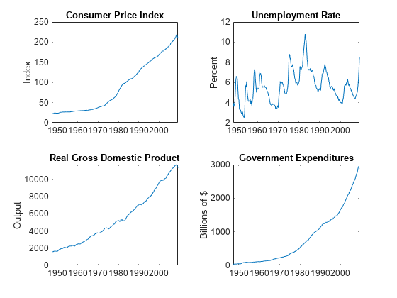
Load the Data_USEconModel data set. Compute the real GDP.

load Data_USEconModel
DataTimeTable.RGDP = DataTimeTable.GDP./DataTimeTable.GDPDEF*100;

Plot all variables on separate plots.

figure
tiledlayout(2,2)
nexttile
plot(DataTimeTable.Time,DataTimeTable.CPIAUCSL);
ylabel("Index")
title("Consumer Price Index")
nexttile
plot(DataTimeTable.Time,DataTimeTable.UNRATE);
ylabel("Percent")
title("Unemployment Rate")
nexttile
plot(DataTimeTable.Time,DataTimeTable.RGDP);
ylabel("Output")
title("Real Gross Domestic Product")
nexttile
plot(DataTimeTable.Time,DataTimeTable.GCE);
ylabel("Billions of $")
title("Government Expenditures")

Figure contains 4 axes objects. Axes object 1 with title Consumer Price Index, ylabel Index contains an object of type line. Axes object 2 with title Unemployment Rate, ylabel Percent contains an object of type line. Axes object 3 with title Real Gross Domestic Product, ylabel Output contains an object of type line. Axes object 4 with title Government Expenditures, ylabel Billions of $ contains an object of type line.

Stabilize the CPI, GDP, and GCE by converting each to a series of growth rates. Synchronize the unemployment rate series with the others by removing its first observation.

varnames = ["CPIAUCSL" "RGDP" "GCE"];
DTT = varfun(@price2ret,DataTimeTable,InputVariables=varnames);
DTT.Properties.VariableNames = varnames;
DTT.UNRATE = DataTimeTable.UNRATE(2:end);

Make the time base regular.

dt = DTT.Time;
dt = dateshift(dt,"start","quarter");
DTT.Time = dt;

Expand the GCE rate series to a matrix that includes the first lagged series through the fourth lag series.

RGCELags = lagmatrix(DTT,1:4,DataVariables="GCE");
DTT = [DTT RGCELags];
DTT = rmmissing(DTT);

Create a default VAR(4) model by using the shorthand syntax. Specify the response variable names.

Mdl = varm(3,4);
Mdl.SeriesNames = ["CPIAUCSL" "UNRATE" "RGDP"];

Estimate the model using the entire sample. Specify the GCE and its lags as exogenous predictor data for the regression component.

prednames = contains(DTT.Properties.VariableNames,"GCE");
EstMdl = estimate(Mdl,DTT,PredictorVariables=prednames);

Infer innovations from the estimated model. Supply the predictor data. Return the loglikelihood objective function value.

[Tbl,logL] = infer(EstMdl,DTT,PredictorVariables=prednames);
size(Tbl)
ans = 1×2

   240    11

head(Tbl)
    Time      CPIAUCSL        RGDP          GCE        UNRATE     Lag1GCE       Lag2GCE       Lag3GCE       Lag4GCE      CPIAUCSL_Residuals    UNRATE_Residuals    RGDP_Residuals
    _____    __________    __________    __________    ______    __________    __________    __________    __________    __________________    ________________    ______________

    Q1-49    0.00041815    -0.0031645      0.036603     6.2        0.047147       0.04948       0.04193      0.054347        0.0053457               0.6564          -0.0053201  
    Q2-49    -0.0071324      0.011385    -0.0021164     6.6        0.036603      0.047147       0.04948       0.04193        0.0088626            -0.034796            0.010153  
    Q3-49    -0.0059122     -0.010366     -0.012793     6.6      -0.0021164      0.036603      0.047147       0.04948        0.0029402              0.11695            -0.02318  
    Q4-49     0.0012698      0.040091     -0.021693     6.3       -0.012793    -0.0021164      0.036603      0.047147        0.0040774              -0.2343            0.026583  
    Q1-50      0.010101      0.029649      0.010905     5.4       -0.021693     -0.012793    -0.0021164      0.036603        0.0046233             -0.18043           0.0091538  
    Q2-50       0.01908       0.03844    -0.0043478     4.4        0.010905     -0.021693     -0.012793    -0.0021164         0.015141             -0.34049            0.019797  
    Q3-50      0.025954      0.017994      0.075508     4.3      -0.0043478      0.010905     -0.021693     -0.012793        0.0041785              0.87368           -0.011263  
    Q4-50      0.035395       0.01197       0.14807     3.4        0.075508    -0.0043478      0.010905     -0.021693         0.011772             -0.49694          -0.0044563  
logL
logL = 1.7056e+03

Tbl is a 240-by-11 timetable of data and inferred innovations from the estimated model (residuals).

Plot the residuals on separate plots.

idx = endsWith(Tbl.Properties.VariableNames,"_Residuals");
resvars = Tbl.Properties.VariableNames(idx);
titles = "Residuals: " + EstMdl.SeriesNames;

figure
tiledlayout(2,2)
for j = 1:Mdl.NumSeries
    nexttile
    plot(Tbl.Time,Tbl{:,resvars(j)});
    xlabel("Date");
    title(titles(j));
    hold on
    yline(0,"r--");
    hold off
end

Figure contains 3 axes objects. Axes object 1 with title Residuals: CPIAUCSL, xlabel Date contains 2 objects of type line, constantline. Axes object 2 with title Residuals: UNRATE, xlabel Date contains 2 objects of type line, constantline. Axes object 3 with title Residuals: RGDP, xlabel Date contains 2 objects of type line, constantline.

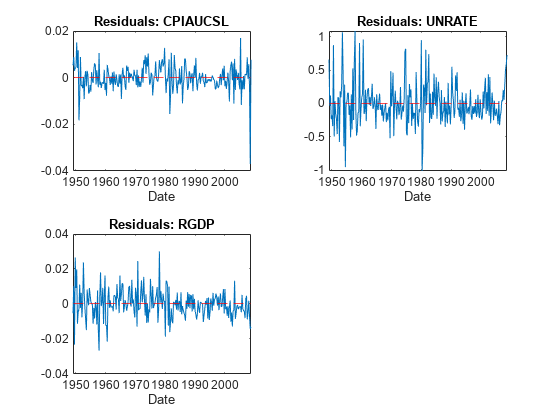
The residuals corresponding to the CPI and GDP growth rates exhibit heteroscedasticity because the CPI series appears to cycle through periods of higher and lower variance. Also, the first half of the GDP series seems to have higher variance than the latter half.

Input Arguments

collapse all

VAR model, specified as a varm model object created by varm or estimate. Mdl must be fully specified.

Response data, specified as a numobs-by-numseries numeric matrix or a numobs-by-numseries-by-numpaths numeric array.

numobs is the sample size. numseries is the number of response series (Mdl.NumSeries). numpaths is the number of response paths.

Rows correspond to observations, and the last row contains the latest observation. Y represents the continuation of the presample response series in Y0.

Columns must correspond to the response variable names in Mdl.SeriesNames.

Pages correspond to separate, independent numseries-dimensional paths. Among all pages, responses in a particular row occur at the same time.

Data Types: double

Since R2022b

Time series data containing observed response variables yt and, optionally, predictor variables xt for a model with a regression component, specified as a table or timetable with numvars variables and numobs rows.

Each selected response variable is a numobs-by-numpaths numeric matrix, and each selected predictor variable is a numeric vector. Each row is an observation, and measurements in each row occur simultaneously. You can optionally specify numseries response variables by using the ResponseVariables name-value argument, and you can specify numpreds predictor variables by using the PredictorVariables name-value argument.

Paths (columns) within a particular response variable are independent, but path j of all variables correspond, for j = 1,…,numpaths.

If Tbl1 is a timetable, it must represent a sample with a regular datetime time step (see isregular), and the datetime vector Tbl1.Time must be ascending or descending.

If Tbl1 is a table, the last row contains the latest observation.

Name-Value Arguments

Specify optional pairs of arguments as Name1=Value1,...,NameN=ValueN, where Name is the argument name and Value is the corresponding value. Name-value arguments must appear after other arguments, but the order of the pairs does not matter.

Before R2021a, use commas to separate each name and value, and enclose Name in quotes.

Example: infer(Mdl,Y,Y0=PS,X=Exo) computes the residuals of the VAR(p) model Mdl at the matrix of response data Y, and specifies the matrix of presample response data PS and the matrix of exogenous predictor data Exo.

Since R2022b

Variables to select from Tbl1 to treat as response variables yt, specified as one of the following data types:

  • String vector or cell vector of character vectors containing numseries variable names in Tbl1.Properties.VariableNames

  • A length numseries vector of unique indices (integers) of variables to select from Tbl1.Properties.VariableNames

  • A length numvars logical vector, where ResponseVariables(j) = true selects variable j from Tbl1.Properties.VariableNames, and sum(ResponseVariables) is numseries

The selected variables must be numeric vectors (single path) or matrices (columns represent multiple independent paths) of the same width, and cannot contain missing values (NaN).

If the number of variables in Tbl1 matches Mdl.NumSeries, the default specifies all variables in Tbl1. If the number of variables in Tbl1 exceeds Mdl.NumSeries, the default matches variables in Tbl1 to names in Mdl.SeriesNames.

Example: ResponseVariables=["GDP" "CPI"]

Example: ResponseVariables=[true false true false] or ResponseVariable=[1 3] selects the first and third table variables as the response variables.

Data Types: double | logical | char | cell | string

Presample responses that provide initial values for the model Mdl, specified as a numpreobs-by-numseries numeric matrix or a numpreobs-by-numseries-by-numprepaths numeric array. Use Y0 only when you supply a numeric array of response data Y.

numpreobs is the number of presample observations. numprepaths is the number of presample response paths.

Each row is a presample observation, and measurements in each row, among all pages, occur simultaneously. The last row contains the latest presample observation. Y0 must have at least Mdl.P rows. If you supply more rows than necessary, infer uses the latest Mdl.P observations only.

Each column corresponds to the response series associated with the respective response series in Y.

Pages correspond to separate, independent paths.

  • If Y0 is a matrix, infer applies it to each path (page) in Y. Therefore, all paths in Y derive from common initial conditions.

  • Otherwise, infer applies Y0(:,:,j) to Y(:,:,j). Y0 must have at least numpaths pages, and infer uses only the first numpaths pages.

By default, infer uses the first Mdl.P observations, for example, Y(1:Mdl.P,:), as a presample. This action reduces the effective sample size.

Data Types: double

Since R2022b

Presample data that provides initial values for the model Mdl, specified as a table or timetable, the same type as Tbl1, with numprevars variables and numpreobs rows.

Each row is a presample observation, and measurements in each row, among all paths, occur simultaneously. numpreobs must be at least Mdl.P. If you supply more rows than necessary, infer uses the latest Mdl.P observations only.

Each variable is a numpreobs-by-numprepaths numeric matrix. Variables correspond to the response series associated with the respective response variable in Tbl1. To control presample variable selection, see the optional PresampleResponseVariables name-value argument.

For each variable, columns are separate, independent paths.

  • If variables are vectors, infer applies them to each path in Tbl1 to produce the corresponding residuals in Tbl2. Therefore, all response paths derive from common initial conditions.

  • Otherwise, for each variable ResponseK and each path j, infer applies Presample.ResponseK(:,j) to produce Tbl2.ResponseK(:,j). Variables must have at least numpaths columns, and infer uses only the first numpaths columns.

If Presample is a timetable, all the following conditions must be true:

  • Presample must represent a sample with a regular datetime time step (see isregular).

  • The inputs Tbl1 and Presample must be consistent in time such that Presample immediately precedes Tbl1 with respect to the sampling frequency and order.

  • The datetime vector of sample timestamps Presample.Time must be ascending or descending.

If Presample is a table, the last row contains the latest presample observation.

By default, infer uses the first or earliest Mdl.P observations in Tbl1 as a presample, and then it fits the model to the remaining numobs – Mdl.P observations. This action reduces the effective sample size.

Since R2022b

Variables to select from Presample to use for presample data, specified as one of the following data types:

  • String vector or cell vector of character vectors containing numseries variable names in Presample.Properties.VariableNames

  • A length numseries vector of unique indices (integers) of variables to select from Presample.Properties.VariableNames

  • A length numvars logical vector, where PresampleResponseVariables(j) = true selects variable j from Presample.Properties.VariableNames, and sum(PresampleResponseVariables) is numseries

The selected variables must be numeric vectors (single path) or matrices (columns represent multiple independent paths) of the same width, and cannot contain missing values (NaN).

PresampleResponseNames does not need to contain the same names as in Tbl1; infer uses the data in selected variable PresampleResponseVariables(j) as a presample for the response variable corresponding to ResponseVariables(j).

The default specifies the same response variables as those selected from Tbl1 (see ResponseVariables).

Example: PresampleResponseVariables=["GDP" "CPI"]

Example: PresampleResponseVariables=[true false true false] or PresampleResponseVariable=[1 3] selects the first and third table variables for presample data.

Data Types: double | logical | char | cell | string

Predictor data xt for the regression component in the model, specified as a numeric matrix containing numpreds columns. Use X only when you supply a numeric array of response data Y.

numpreds is the number of predictor variables (size(Mdl.Beta,2)).

Each row corresponds to an observation, and measurements in each row occur simultaneously. The last row contains the latest observation. X must have at least as many observations as Y. If you supply more rows than necessary, infer uses only the latest observations. infer does not use the regression component in the presample period.

  • If you specify a numeric array for a presample by using Y0, X must have at least numobs rows (see Y).

  • Otherwise, X must have at least numobsMdl.P observations to account for the default presample removal from Y.

Each column is an individual predictor variable. All predictor variables are present in the regression component of each response equation.

infer applies X to each path (page) in Y; that is, X represents one path of observed predictors.

By default, infer excludes the regression component, regardless of its presence in Mdl.

Data Types: double

Since R2022b

Variables to select from Tbl1 to treat as exogenous predictor variables xt, specified as one of the following data types:

  • String vector or cell vector of character vectors containing numpreds variable names in Tbl1.Properties.VariableNames

  • A length numpreds vector of unique indices (integers) of variables to select from Tbl1.Properties.VariableNames

  • A length numvars logical vector, where PredictorVariables(j) = true selects variable j from Tbl1.Properties.VariableNames, and sum(PredictorVariables) is numpreds

The selected variables must be numeric vectors and cannot contain missing values (NaN).

By default, infer excludes the regression component, regardless of its presence in Mdl.

Example: PredictorVariables=["M1SL" "TB3MS" "UNRATE"]

Example: PredictorVariables=[true false true false] or PredictorVariable=[1 3] selects the first and third table variables to supply the predictor data.

Data Types: double | logical | char | cell | string

Note

  • NaN values in Y, Y0, and X indicate missing values. infer removes missing values from the data by list-wise deletion.

    1. If Y is a 3-D array, then infer horizontally concatenates the pages of Y to form a numobs-by-(numpaths*numseries + numpreds) matrix.

    2. If a regression component is present, then infer horizontally concatenates X to Y to form a numobs-by-numpaths*numseries + 1 matrix. infer assumes that the last rows of each series occur at the same time.

    3. infer removes any row that contains at least one NaN from the concatenated data.

    4. infer applies steps 1 and 3 to the presample paths in Y0.

    This process ensures that the inferred output innovations of each path are the same size and are based on the same observation times. In the case of missing observations, the results obtained from multiple paths of Y can differ from the results obtained from each path individually.

    This type of data reduction reduces the effective sample size.

  • infer issues an error when any table or timetable input contains missing values.

Output Arguments

collapse all

Inferred multivariate innovations series, returned as either a numeric matrix, or as a numeric array that contains columns and pages corresponding to Y. infer returns E only when you supply a matrix of response data Y.

  • If you specify Y0, then E has numobs rows (see Y).

  • Otherwise, E has numobsMdl.P rows to account for the presample removal.

Since R2022b

Inferred multivariate innovations series and other variables, returned as a table or timetable, the same data type as Tbl1. infer returns Tbl2 only when you supply the input Tbl1.

Tbl2 contains the inferred innovation paths E from evaluating the model Mdl at the paths of selected response variables Y, and it contains all variables in Tbl1. infer names the innovation variable corresponding to variable ResponseJ in Tbl1 ResponseJ_Residuals. For example, if one of the selected response variables for estimation in Tbl1 is GDP, Tbl2 contains a variable for the residuals in the response equation of GDP with the name GDP_Residuals.

If you specify presample response data, Tbl2 and Tbl1 have the same number of rows, and their rows correspond. Otherwise, because infer removes initial observations from Tbl1 for the required presample by default, Tbl2 has numobs – Mdl.P rows to account for that removal.

If Tbl1 is a timetable, Tbl1 and Tbl2 have the same row order, either ascending or descending.

Loglikelihood objective function value, returned as a numeric scalar or a numpaths-element numeric vector. logL(j) corresponds to the response path in Y(:,:,j) or the path (column) j of the selected response variables of Tbl1.

Algorithms

Suppose Y, Y0, and X are the response, presample response, and predictor data specified by the numeric data inputs in Y, Y0, and X, or the selected variables from the input tables or timetables Tbl1 and Presample.

  • infer infers innovations by evaluating the VAR model Mdl, specifically,

    ε^t=Φ^(L)ytc^β^xtδ^t.

  • infer uses this process to determine the time origin t0 of models that include linear time trends.

    • If you do not specify Y0, then t0 = 0.

    • Otherwise, infer sets t0 to size(Y0,1)Mdl.P. Therefore, the times in the trend component are t = t0 + 1, t0 + 2,..., t0 + numobs, where numobs is the effective sample size (size(Y,1) after infer removes missing values). This convention is consistent with the default behavior of model estimation in which estimate removes the first Mdl.P responses, reducing the effective sample size. Although infer explicitly uses the first Mdl.P presample responses in Y0 to initialize the model, the total number of observations in Y0 and Y (excluding missing values) determines t0.

References

[1] Hamilton, James D. Time Series Analysis. Princeton, NJ: Princeton University Press, 1994.

[2] Johansen, S. Likelihood-Based Inference in Cointegrated Vector Autoregressive Models. Oxford: Oxford University Press, 1995.

[3] Juselius, K. The Cointegrated VAR Model. Oxford: Oxford University Press, 2006.

[4] Lütkepohl, H. New Introduction to Multiple Time Series Analysis. Berlin: Springer, 2005.

Version History

Introduced in R2017a

expand all