armafevd
Generate or plot ARMA model forecast error variance decomposition (FEVD)
Syntax
Description
The armafevd function returns or plots the forecast error variance decomposition of the variables in a univariate or vector (multivariate) autoregressive moving average (ARMA or VARMA) model specified by arrays of coefficients or lag operator polynomials.
Alternatively, you can return an FEVD from a fully specified (for example, estimated) model object by using a function in this table.
The FEVD provides information about the relative importance of each innovation in affecting the forecast error variance of all variables in the system. In contrast, the impulse response function (IRF) traces the effects of an innovation shock to one variable on the response of all variables in the system. To estimate IRFs of univariate or multivariate ARMA models, see armairf.
armafevd(
plots, in separate figures, the FEVD of the time series variables that compose an
ARMA(p,q) model, with input autoregressive (AR)
and moving average (MA) coefficients. Each figure corresponds to a variable and contains a
line plot for each time series variable. The line plots are the FEVDs of that variable,
over the forecast horizon, resulting from a one-standard-deviation innovation shock
applied to all variables in the system at time 0.ar0,ma0)
The armafevd function:
Accepts vectors or cell vectors of matrices in difference-equation notation
Accepts
LagOplag operator polynomials corresponding to the AR and MA polynomials in lag operator notationAccommodates time series models that are univariate or multivariate, stationary or integrated, structural or in reduced form, and invertible or noninvertible
Assumes that the model constant c is 0
armafevd(
plots the ar0,ma0,Name=Value)numVars FEVDs with additional options specified by one or
more name-value arguments. For example, NumObs=10,Method="generalized"
specifies a 10-period forecast horizon and the estimation of the generalized FEVD.
armafevd(
plots to the axes specified in ax,___)ax instead of
the axes in new figures. The option ax can precede any of the input argument
combinations in the previous syntaxes.
Examples
Plot the FEVD of the univariate ARMA(2,1) model
Create vectors for the autoregressive and moving average coefficients as you encounter them in the model, which is expressed in difference-equation notation.
AR0 = [0.3 -0.1];
MA0 = 0.05;
Plot the orthogonalized FEVD of .
armafevd(AR0,MA0);
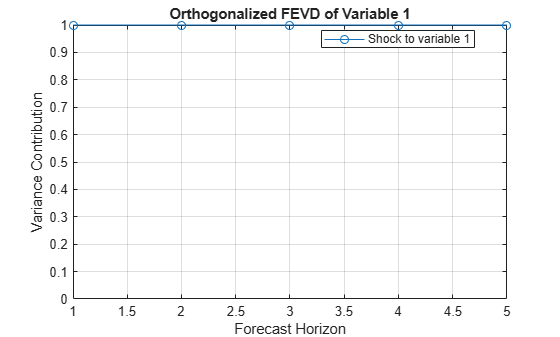
Because is univariate, the FEVD is trivial.
Plot the FEVD of the VARMA(3,1) model
where and .
The VARMA model is in difference-equation notation because the current response is isolated from all other terms in the equation.
Create a cell vector containing the VAR matrix coefficients. The position of the coefficient matrix in the cell vector determines its lag. Therefore, specify a 3-by-3 matrix of zeros as the second element of the vector.
var0 = {[-0.5 0.2 0.1; 0.3 0.1 -0.1; -0.4 0.2 0.05],...
    zeros(3),...
    [-0.05 0.02 0.01; 0.1 0.01 0.001; -0.04 0.02 0.005]};
Create a cell vector containing the VMA matrix coefficients.
vma0 = {[-0.02 0.03 0.3; 0.003 0.001 0.01; 0.3 0.01 0.01]};Plot the orthogonalized FEVDs of the VARMA model.
armafevd(var0,vma0);
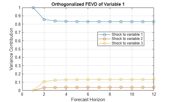
armafevd returns three figures. Figure k contains the generalized FEVD of variable k to a shock applied to all other variables at time 0.
You can attribute most of the forecast error variance of variable 1 to a shock to variable 1. A shock to variable 2 does not contribute much to the forecast error variance of variable 1.
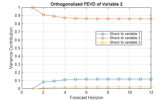
You can attribute most of the forecast error variance of variable 2 to a shock to variable 2. A shock to variable 3 does not contribute much to the forecast error variance of variable 2.
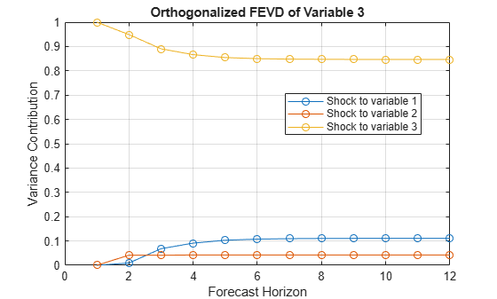
You can attribute most of the forecast error variance of variable 3 to a shock to variable 3. A shock to variable 2 does not contribute much to the forecast error variance of variable 3.
Plot the entire FEVD of the structural VARMA(8,4) model
where and .
The VARMA model is in lag operator notation because the response and innovation vectors are on opposite sides of the equation.
Create a cell vector containing the VAR matrix coefficients. Because this model is a structural model in lag operator notation, start with the coefficient of and enter the rest in order by lag. Construct a vector that indicates the degree of the lag term for the corresponding coefficients (the structural-coefficient lag is 0).
var0 = {[1 0.2 -0.1; 0.03 1 -0.15; 0.9 -0.25 1],...
    -[-0.5 0.2 0.1; 0.3 0.1 -0.1; -0.4 0.2 0.05],...
    -[-0.05 0.02 0.01; 0.1 0.01 0.001; -0.04 0.02 0.005]};
var0Lags = [0 4 8];
Create a cell vector containing the VMA matrix coefficients. Because this model is in lag operator notation, start with the coefficient of and enter the rest in order by lag. Construct a vector that indicates the degree of the lag term for the corresponding coefficients.
vma0 = {eye(3),...
    [-0.02 0.03 0.3; 0.003 0.001 0.01; 0.3 0.01 0.01]};
vma0Lags = [0 4];
Construct separate lag operator polynomials that describe the VAR and VMA components of the VARMA model.
VARLag = LagOp(var0,Lags=var0Lags);
VMALag = LagOp(vma0,Lags=vma0Lags);
Plot the generalized FEVDs of the VARMA model.
armafevd(VARLag,VMALag,Method="generalized");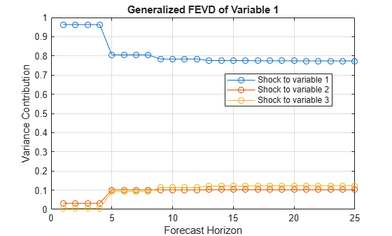
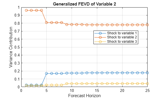
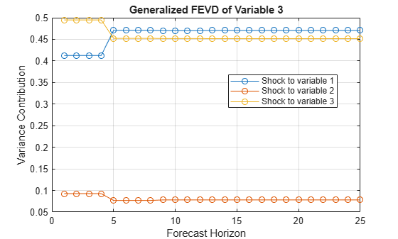
armafevd returns three figures. Figure k contains the generalized FEVD of variable k to a shock applied to all other variables at time 0.
You can attribute most of the forecast error variance of variable 1 to a shock to variable 1. Shocks to variables 2 and 3 contribute similarly to the forecast error variance of variable 1.
You can attribute most of the forecast error variance of variable 2 to a shock to variable 2. A shock to variable 3 does not contribute much to the forecast error variance of variable 2.
You can attribute most of the forecast error variance of variable 3 to shocks to variables 1 and 3, each contributing similar amounts. A shock to variable 2 does not contribute much to the forecast error variance of variable 3.
Compute the generalized FEVDs of the two-dimensional VAR(3) model
In the equation, , , and, for all t, is Gaussian with mean zero and covariance matrix
Create a cell vector of matrices for the autoregressive coefficients as you encounter them in the model as expressed in difference-equation notation. Specify the innovation covariance matrix.
AR1 = [1 -0.2; -0.1 0.3];
AR2 = -[0.75 -0.1; -0.05 0.15];
AR3 = [0.55 -0.02; -0.01 0.03];
ar0 = {AR1 AR2 AR3};

InnovCov = [0.5 -0.1; -0.1 0.25];
Compute the generalized FEVDs of . Because no MA terms exist, specify an empty array ([]) for the second input argument.
Y = armafevd(ar0,[],Method="generalized",InnovCov=InnovCov);
size(Y)
ans = 1×3
31 2 2
Y(10,1,2)
ans =
0.1302
Y is a 31-by-2-by-2 array of FEVDs. Rows correspond to times 1 through 31 in the forecast horizon, columns correspond to the variables that armafevd shocks at time 0, and pages correspond to the FEVD of the variables in the system. For example, the contribution to the forecast error variance of variable 2 at time 10 in the forecast horizon, attributable to a shock to variable 1, is Y(10,1,2) = 0.1302.
armafevd satisfies the stopping criterion after 31 periods. You can specify to stop sooner using the NumObs name-value argument. This practice is beneficial when the system has many variables.
Compute and display the generalized FEVDs for the first 10 periods.
Y10 = armafevd(ar0,[],Method="generalized",InnovCov=InnovCov, ...
    NumObs=10)
Y10 =
Y10(:,:,1) =

    1.0000    0.0800
    0.9912    0.1238
    0.9863    0.1343
    0.9863    0.1341
    0.9873    0.1294
    0.9874    0.1313
    0.9864    0.1342
    0.9864    0.1343
    0.9866    0.1336
    0.9867    0.1336


Y10(:,:,2) =

    0.0800    1.0000
    0.1157    0.9838
    0.1235    0.9737
    0.1236    0.9737
    0.1237    0.9736
    0.1264    0.9709
    0.1296    0.9679
    0.1298    0.9677
    0.1298    0.9677
    0.1302    0.9673
Y10 is a 10-by-2-by-2 array of FEVDs. Rows correspond to times 1 through 10 in the forecast horizon. In all FEVDs, the contributions appear to stabilize before 10 periods elapse.
For each variable (page), compute the row sums.
sum(Y10,2)
ans =
ans(:,:,1) =

    1.0800
    1.1150
    1.1206
    1.1204
    1.1167
    1.1187
    1.1206
    1.1207
    1.1202
    1.1203


ans(:,:,2) =

    1.0800
    1.0995
    1.0972
    1.0973
    1.0973
    1.0973
    1.0975
    1.0975
    1.0975
    1.0975
For generalized FEVDs, forecast error variance contributions at each period in the forecast horizon do not necessarily sum to one. This characteristic is in contrast to orthogonalized FEVDs, in which all rows sum to one.
Input Arguments
Name-Value Arguments
Output Arguments
More About
Tips
To accommodate structural ARMA(p,q) models, supply
LagOplag operator polynomials for the input argumentsar0andma0. To specify a structural coefficient when you callLagOp, set the corresponding lag to 0 by using theLagsname-value argument.For orthogonalized multivariate FEVDs, arrange the variables according to Wold causal ordering [3]:
The first variable (corresponding to the first row and column of both
ar0andma0) is most likely to have an immediate impact (t = 0) on all other variables.The second variable (corresponding to the second row and column of both
ar0andma0) is most likely to have an immediate impact on the remaining variables, but not the first variable.In general, variable j (corresponding to row j and column j of both
ar0andma0) is the most likely to have an immediate impact on the lastnumVars– j variables, but not the previous j – 1 variables.
Algorithms
armafevdplots FEVDs only when it returns no output arguments orh.If
Methodis"orthogonalized",armafevdorthogonalizes the innovation shocks by applying the Cholesky factorization of the innovations covariance matrixInnovCov. The covariance of the orthogonalized innovation shocks is the identity matrix, and the FEVD of each variable sums to one, that is, the sum along any row ofYis one. Therefore, the orthogonalized FEVD represents the proportion of forecast error variance attributable to various shocks in the system. However, the orthogonalized FEVD generally depends on the order of the variables.If
Methodis"generalized":The resulting FEVD is invariant to the order of the variables.
The resulting FEVD is not based on an orthogonal transformation.
The resulting FEVD of a variable sums to one only when
InnovCovis diagonal [4].
Therefore, the generalized FEVD represents the contribution to the forecast error variance of equation-wise shocks to the variables in the system.
If
InnovCovis a diagonal matrix, then the resulting generalized and orthogonalized FEVDs are identical. Otherwise, the resulting generalized and orthogonalized FEVDs are identical only when the first variable shocks all variables (in other words, all else being the same, both methods yield the same value ofY(:,1,:)).
References
[1] Hamilton, James D. Time Series Analysis. Princeton, NJ: Princeton University Press, 1994.
[2] Lütkepohl, H. "Asymptotic Distributions of Impulse Response Functions and Forecast Error Variance Decompositions of Vector Autoregressive Models." Review of Economics and Statistics. Vol. 72, 1990, pp. 116–125.
[3] Lütkepohl, Helmut. New Introduction to Multiple Time Series Analysis. New York, NY: Springer-Verlag, 2007.
[4] Pesaran, H. H., and Y. Shin. "Generalized Impulse Response Analysis in Linear Multivariate Models." Economic Letters. Vol. 58, 1998, pp. 17–29.
Version History
Introduced in R2018b