Format Multivariate Time Series Data
The first step in multivariate time series analysis is to obtain, inspect, and preprocess data. This topic describes the following:
How to load economic data into MATLAB®
Appropriate data types and structures for multivariate time series analysis functions
Common characteristics of time series data that can warrant transforming the set before proceeding with an analysis
How to partition your data into presample, estimation, and forecast samples.
Multivariate Time Series Data
Two main types of multivariate time series data are:
Response data – Observations from the n-D multivariate time series of responses yt (see Types of Stationary Multivariate Time Series Models).
Exogenous data – Observations from the m-D multivariate time series of predictors xt. Each variable in the exogenous data appears in all response equations by default.
Before specifying any data set as an input to Econometrics Toolbox™ functions, format the data appropriately. Use standard MATLAB commands, or preprocess the data with a spreadsheet program, database program, PERL, or other tool.
You can obtain historical time series data from several freely available sources, such as the St. Louis Federal Reserve Economics Database (known as FRED®): https://research.stlouisfed.org/fred2/. If you have a Datafeed Toolbox™ license, you can use the toolbox functions to access data from various sources.
Load Multivariate Economic Data
The file Data_USEconModel ships with Econometrics Toolbox. It contains time series from FRED.
Load the data into the MATLAB Workspace.
load Data_USEconModelVariables in the workspace include:
Data, a 249-by-14 matrix containing 14 macroeconomic time series observations.DataTable, a 249-by-14 MATLAB table containing the same time series observations.DataTimeTable, a 249-by-14 MATLAB timetable containing the same time series observations, but the observations are timestamped.Description, a character array containing a description of the data series and the key to the labels for each series.series, a 1-by-14 cell array of labels for the time series.
Data, DataTable, and
DataTimeTable contain the same data. However, the tables
enable you to use dot notation to access a variable. For example,
DataTimeTable.UNRATE specifies the unemployment rate series.
All timetables contain the variable Time, which is a
datetime vector of observation timestamps. For more details,
see Create Timetables and Represent Dates and Times in MATLAB.
Display the first and last sampling times and the names of the variables by using
DataTimeTable.
firstperiod = DataTimeTable.Time(1)
lastperiod = DataTimeTable.Time(end)
seriesnames = DataTimeTable.Properties.VariableNames
firstperiod =

  datetime

   Q1-47


lastperiod =

  datetime

   Q1-09


seriesnames =

  1×14 cell array

  Columns 1 through 8

    {'COE'}    {'CPIAUCSL'}    {'FEDFUNDS'}    {'GCE'}    {'GDP'}    {'GDPDEF'}    {'GPDI'}    {'GS10'}

  Columns 9 through 14

    {'HOANBS'}    {'M1SL'}    {'M2SL'}    {'PCEC'}    {'TB3MS'}    {'UNRATE'}
This table describes the variables in DataTimeTable.
| FRED Variable | Description |
|---|---|
COE | Paid compensation of employees in $ billions |
CPIAUCSL
| Consumer price index (CPI) |
FEDFUNDS | Effective federal funds rate |
GCE | Government consumption expenditures and investment in $ billions |
GDP | Gross domestic product (GDP) |
GDPDEF | Gross domestic product in $ billions |
GPDI | Gross private domestic investment in $ billions |
GS10 | Ten-year treasury bond yield |
HOANBS | Nonfarm business sector index of hours worked |
M1SL | M1 money supply (narrow money) |
M2SL | M2 money supply (broad money) |
PCEC | Personal consumption expenditures in $ billions |
TB3MS | Three-month treasury bill yield |
UNRATE | Unemployment rate |
Consider studying the dynamics of the GDP, CPI, and unemployment rate, and suppose government consumption expenditures is an exogenous variable. Create arrays for the response and predictor data. Display the latest observation in each array.
Y = DataTimeTable{:,["CPIAUCSL" "UNRATE" "GDP"]};
x = DataTimeTable.GCE;

lastobsresponse = Y(end,:)
lastobspredictor = x(end)
lastobsresponse =
1.0e+04 *
0.0213 0.0008 1.4090
lastobspredictor =
2.8833e+03Y and x represent one path of observations, and are appropriately formatted for passing to multivariate model object functions. The timestamp information does not apply to the arrays because analyses assume sampling times are evenly spaced.
Multivariate Data Format
You can load response and optional data sets, such as predictor data, into the MATLAB Workspace as numeric arrays, MATLAB tables, or MATLAB timetables. However, you must specify the same data type for each function call.
For numeric arrays, you specify each data set that functions use for a particular purpose as a separate input. Specifically, presample response data is a separate input from in-sample estimation data, and response and predictor data sets are separate array inputs.
For tables and timetables, you specify all contemporaneous data (simultaneous
measurements) functions use for a particular purpose in the same table or timetable.
Specifically, presample and estimation sample data are separate tables of
timetables, but all in-sample response and predictor variables are in the same input
table or timetable. You specify variables to that contain the response and predictor
data using the appropriate variable selection name-value arguments, for example,
ResponseVariables.
The type of variable and problem context determine the format of the data that you supply. For any array containing multivariate time series data:
Row t of the input contains the observations of all variables at time t.
For an array input, column j of the array contains all observations of variable j. MATLAB treats each variable in an array as distinct.
For numeric array data inputs, a matrix of data indicates one sample path. To
create a variable representing one path of length T of response
data, put the data into a T-by-n matrix
Y:
Y(
= yj,t, which is
observation t of response variable j. A single
path of data created for predictor variables, or other variables, has a similar
form.t,j)
For table or timetable data inputs, you specify a single path of data for variable
j by using a numeric vector. Therefore,
Tbl{
is observation t of variable j in the table.
The variable selection name-value arguments determine the type of variable, either
response, predictor, or otherwise.t,j}
You can specify one path of observations as an input to all multivariate model object functions that accept data. Examples of situations in which you supply one path include:
Fit response and predictor data to a VARX model. You supply both a path of response data and a path of predictor data, see
estimate.Initialize a VEC model with a path of presample data for forecasting or simulating paths (see
forecastorsimulate).Obtain a single response path from filtering a path of innovations through a VAR model (see
filter).Generate conditional forecasts from a VAR model given a path of future response data (see
forecast).
For numeric array data inputs, a 3-D array indicates multiple independent sample
paths of data. You can create
T-by-n-by-p array
Y, representing p sample paths of response
data, by stacking single paths of responses (matrices) along the third dimension.
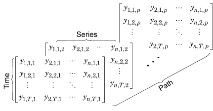
Y(
=
yj,t,k,
which is observation t of response variable j
from path k, k = 1,…,p. All
paths must have the same sample times, and variables among paths must correspond.
For more details, see Multidimensional Arrays.t,j,k)
For table or timetable data inputs, matrix-valued variables indicate multiple independent sample paths of data. Column k of the matrix of each variable represents path k, and all path k of all variables correspond.
You can specify multiple paths of responses or innovations as an input to several multivariate model object functions that accept data. Examples of situations in which you supply multiple paths include:
Initialize a VEC model with multiple paths of presample data for forecasting or simulating multiple paths. Each specified path can represent different initial conditions, from which the functions generate forecasts or simulations.
Obtain multiple response paths from filtering multiple paths of innovations through a VAR model. This process is an alternative way to simulate multiple response paths.
Generate multiple conditional forecast paths from a VAR model given multiple paths of future response data.
estimate does not support the specification of
multiple paths of response data.
Exogenous Data Format
All multivariate model object functions that take exogenous data as an input accept a matrix or variables in an input table or timetable X representing one path of observations in the in-sample period. MATLAB includes all exogenous variables in the regression component of each response equation. For a VAR(p) model, the response equations are:
To configure the regression components of the response
equations, work with the regression coefficient matrix (stored in the
Beta property of the model object) rather than the data.
For more details, see Create VAR Model and Select Exogenous Variables for Response Equations.
Multivariate model object functions do not support multiple paths of predictor data. However, if you specify a path of predictor data and multiple paths of response or innovations data, the function associates the same predictor data to all paths. For example, if you simulate paths of responses from a VARX model and specify multiple paths of presample values, simulate applies the same exogenous data to each generated response path.
Preprocess Data
Your data might have characteristics that violate model assumptions. For example, you can have data with exponential growth, or data from multiple sources at different periodicities. In such cases, preprocess or transform the data to an acceptable form for analysis.
Inspect the data for missing values, which are indicated by
NaNs.For numeric array inputs, object functions use list-wise deletion to remove observations containing at least one missing value. If at least one response or predictor variable has a missing value for a time point (row), MATLAB removes all observations for that time (the entire row of the response and predictor data matrices). Such deletion can have implications on the time base and the effective sample size. Therefore, you should investigate and address any missing values before starting an analysis.
For table or timetable inputs, object functions issue an error when specified data sets contain any missing values.
For data from multiple sources, you must decide how to synchronize the data. Data synchronization can include data aggregation or disaggregation, and the latter can create patterns of missing values. You can address these types of induced missing values by imputing previous values (that is, a missing value is unchanged from its previous value), or by interpolating them from neighboring values.
If the time series are variables in a timetable, then you can synchronize your data by using
synchronize.For time series exhibiting exponential growth, you can preprocess the data by taking the logarithm of the growing series. In some cases, you must apply the first difference of the result (see
price2ret). For more details on stabilizing time series, see Unit Root Nonstationarity. For an example, see VAR Model Case Study.
Note
If you apply the first difference of a series, the resulting series is one observation shorter than the original series. If you apply the first difference of only some time series in a data set, truncate the other series so that all have the same length, or pad the differenced series with initial values.
Time Base Partitions for Estimation
When you fit a time series model to data, lagged terms in the model require initialization, usually with observations at the beginning of the sample. Also, to measure the quality of forecasts from the model, you must hold out data at the end of your sample from estimation. Therefore, before analyzing the data, partition the time base into three consecutive, disjoint intervals:
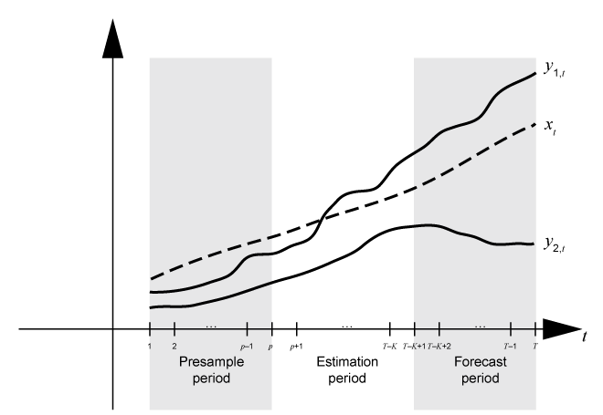
Three time base partitions for multivariate vector autoregression (VAR) and vector error-correction (VEC) models are the presample, estimation, and forecast periods.
Presample period – Contains data used to initialize lagged values in the model. Both VAR(p) and VEC(p–1) models require a presample period containing at least p multivariate observations. For example, if you plan to fit a VAR(4) model, the conditional expected value of yt, given its history, contains yt – 1, yt – 2, yt – 3, and yt – 4. The conditional expected value of y5 is a function of y1, y2, y3, and y4. Therefore, the likelihood contribution of y5 requires y1–y4, which implies that data does not exist for the likelihood contributions of y1–y4. In this case, model estimation requires a presample period of at least four time points.
Estimation period — Contains the observations to which the model is explicitly fit. The number of observations in the estimation sample is the effective sample size. For parameter identifiability, the effective sample size should be at least the number of parameters being estimated.
Forecast period — Optional period during which forecasts are generated, known as the forecast horizon. This partition contains holdout data for model predictability validation.
Suppose yt is a 2-D response series and xt is a 1-D exogenous series. Consider fitting a VARX(p) model of yt to the response data in the T-by-2 matrix Y and the exogenous data in the T-by-1 vector x. Also, you want the forecast horizon to have length K (that is, you want to hold out K observations at the end of the sample to compare to the forecasts from the fitted model). This figure shows the time base partitions for model estimation.
This figure shows portions of the arrays that correspond to numeric array input
arguments of the estimate function.
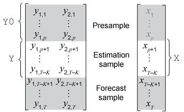
Yis the required input for specifying the response data to which the model is fit. Alternatively, you can specify estimation sample response and predictor data in a table or regular timetableTbl.Y0is an optional name-value argument for specifying the presample response data in a numeric matrix.Y0must have at least p rows. To initialize the model,estimateuses only the latest p observationsY0((end –. Similarly, you can supply optional presample data in a table or timetable by using thep+ 1):end,:)Presamplename-value argument. IfPresampleis a timetable, its timestamps must directly precede those ofTbl, and the sampling frequency between the timestamps must match.Xis an optional name-value argument for specifying exogenous data for the linear regression component. By default,estimateexcludes a regression component from the model, regardless of the value of the regression coefficientBetaof thearimamodel template for estimation. Alternatively, you can select predictor variables from the input table or timetable of estimation sample dataTblby using thePredictorVariablesname-value argument.
If you do not specify presample data (Y0 or
Presample), estimate removes
observations 1 through p from the estimation sample to initialize
the model, and then fits the model to the rest of the data, for example,
Y((. That is,
p + 1):end,:)estimate infers the presample and estimation periods from
the input estimation sample data. Although estimate extracts
the presample from the estimation sample by default, you can extract the presample
from the data and specify it using the name-value argument appropriate for the data
type, which ensures that estimate initializes and fits the
model to your specifications.
If you specify predictor data (X or
PredictorVariables name-value arguments):
For numeric array input data,
estimatesynchronizesXandYwith respect to the last observation in the arrays (T – K in the previous figure), and applies only the required number of observations to the regression component. This action implies thatXcan have more rows thatY.For table or timetable input data, all variables are synchronized because the estimation sample data is one input.
For numeric array input data, if you also specify presample data,
estimateuses only the latest exogenous data observations required to fit the model (observations J + 1 through T – K in the previous figure).estimateignores presample exogenous data. This fact doesn't apply to table or timetable input data.
If you plan to validate the predictive power of the fitted model, you must extract the forecast sample from your data set before estimation.
Partition Multivariate Time Series Data for Estimation
Consider fitting a VAR(4) model to the data and variables in Load Multivariate Economic Data, and holding out the last 2 years of data to validate the predictive power of the fitted model.
Load the data. Create a timetable containing the predictor and response variables
load Data_USEconModel

responsenames = ["CPIAUCSL" "UNRATE" "GDP"];
predictorname = "GCE";
TT = DataTimeTable(:,[responsenames predictorname]);
Identify all rows in the timetable containing at least one missing observation (NaN).
whichmissing = ismissing(TT);
idxvar = sum(whichmissing) > 0;
hasmissing = TT.Properties.VariableNames(idxvar)
hasmissing = 1×1 cell array
    {'UNRATE'}
wheremissing = find(whichmissing(:,idxvar) > 0)
wheremissing = 4×1

     1
     2
     3
     4
The unemployment rate is missing the first year of data in the sample.
Remove the observations (rows) with the leading missing values from the data.
TT = rmmissing(TT);
rmmissing uses listwise deletion to remove all rows from the input timetable containing at least one missing observation.
A VAR(4) model requires 4 presample responses, and the forecast sample requires 2 years (8 quarters) of data. Partition the response data into presample, estimation, and forecast sample variables. Partition the predictor data into estimation and forecast sample variables (presample predictor data is not considered estimation).
p = 4;              % Num. presample observations
fh = 8;             % Forecast horizon
T = size(TT,1);      % Total sample size
eT = T - p - fh;    % Effective sample size

idxpre = 1:p;
idxest = (p + 1):(T - fh);
idxfor = (T - fh + 1):T;

Y0 = TT{idxpre,responsenames};  % Presample responses
YF = TT{idxfor,responsenames};  % Forecast sample responses
Y = TT{idxest,responsenames};   % Estimation sample responses

xf = TT{idxfor,predictorname};
x = TT{idxest,predictorname};
When estimating the model using estimate, specify a varm model template representing a VAR(4) model and the estimation sample response data Y as inputs. Specify the presample response data Y0 to initialize the model by using the 'Y0' name-value pair argument, and specify the estimation sample predictor data x by using the 'X' name-value pair argument. Y and x are synchronized data sets, while Y0 occurs during the previous four periods before the estimation sample starts.
After estimation, you can forecast the model using forecast by specifying the estimated VARX(4) model object returned by estimate, the forecast horizon fh, and estimation sample response data Y to initialize the model for forecasting. Specify the forecast sample predictor data xf for the model regression component by using the 'X' name-value pair argument. Determine the predictive power of the estimation model by comparing the forecasts to the forecast sample response data YF.