VAR Model Case Study
This example shows how to analyze a VAR model.
Overview of Case Study
This section contains an example of the workflow described in VAR Model Workflow. The example uses three time series: GDP, M1 money supply, and the 3-month T-bill rate. The example shows:
Loading and transforming the data for stationarity
Partitioning the transformed data into presample, estimation, and forecast intervals to support a backtesting experiment
Making several models
Fitting the models to the data
Deciding which of the models is best
Making forecasts based on the best model
Load and Transform Data
The file Data_USEconModel ships with Econometrics Toolbox™ software. The file contains time series from the Federal Reserve Bank of St. Louis Economics Data (FRED) database in a tabular array. This example uses three of the time series:
GDP (
GDP)M1 money supply (
M1SL)3-month T-bill rate (
TB3MS)
Load the data set. Create a variable for real GDP.
load Data_USEconModel
DataTimeTable.RGDP = DataTimeTable.GDP./DataTimeTable.GDPDEF*100;
Plot the data to look for trends.
figure
tiledlayout(3,1)
nexttile
plot(DataTimeTable.Time,DataTimeTable.RGDP);
title("Real GDP")
grid on
nexttile
plot(DataTimeTable.Time,DataTimeTable.M1SL);
title("M1")
grid on
nexttile
plot(DataTimeTable.Time,DataTimeTable.TB3MS)
title("3-mo T-bill")
grid on
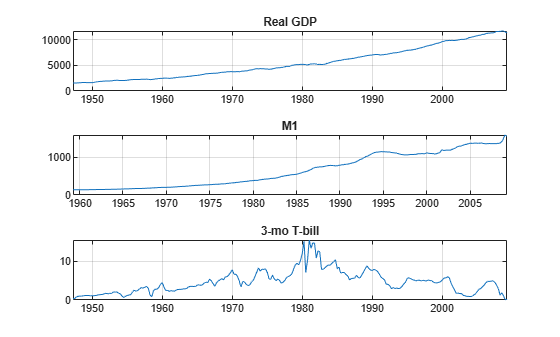
The real GDP and M1 data appear to grow exponentially, while the T-bill returns show no exponential growth. To counter the trends in real GDP and M1, take a difference of the logarithms of the data. Also, stabilize the T-bill series by taking the first difference. Synchronize the date series so that the data has the same number of rows for each column.
rgdpg = price2ret(DataTimeTable.RGDP);
m1slg = price2ret(DataTimeTable.M1SL);
dtb3ms = diff(DataTimeTable.TB3MS);
Data = array2timetable([rgdpg m1slg dtb3ms],...
    RowTimes=DataTimeTable.Time(2:end),VariableNames=["RGDPRate" "M1SLRate" "TB3MSChng"]);
seriesnames = ["Real GDP Rate","M1 Rate","3-mo T-bill Change"];

figure
tiledlayout(3,1)
for j = 1:3
    nexttile
    plot(Data.Time,Data{:,j});
    title(seriesnames(j))
    grid on
end
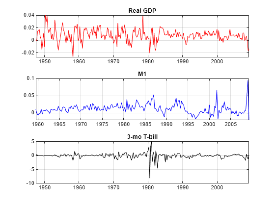
The scale of the first two columns is about 100 times smaller than the third. Multiply the first two columns by 100 so that the time series are all roughly on the same scale. This scaling makes it easy to plot all the series on the same plot. More importantly, this type of scaling makes optimizations more numerically stable (for example, maximizing loglikelihoods).
Data{:,1:2} = 100*Data{:,1:2};
figure
plot(Data.Time,Data.Variables,LineWidth=2);
grid on
legend(seriesnames) 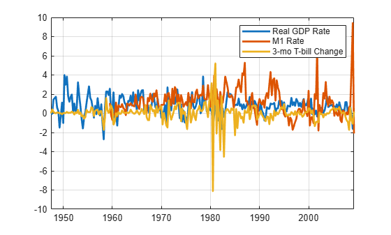
Select and Fit the Models
You can select many different models for the data. This example uses four models.
VAR(2) with diagonal autoregressive
VAR(2) with full autoregressive
VAR(4) with diagonal autoregressive
VAR(4) with full autoregressive
Remove all missing values from the beginning of the series.
Data = rmmissing(Data);
Create the four models.
numseries = 3;
dnan = diag(nan(numseries,1));
VAR2diag = varm(AR={dnan dnan},SeriesNames=seriesnames);
VAR2full = varm(numseries,2);
VAR2full.SeriesNames = seriesnames;
VAR4diag = varm(AR={dnan dnan dnan dnan},SeriesNames=seriesnames);
VAR4full = varm(numseries,4);
VAR4full.SeriesNames = seriesnames;
The matrix dnan is a diagonal matrix with NaN values along its main diagonal. In general, missing values specify the presence of the parameter in the model, and indicate that the parameter needs to be fit to data. MATLAB® holds the off diagonal elements, 0, fixed during estimation. In contrast, the specifications for VAR2full and VAR4full have matrices composed of NaN values. Therefore, estimate fits full matrices for autoregressive matrices.
To assess the quality of the models, create index vectors that divide the response data into three periods: presample, estimation, and forecast. Fit the models to the estimation data, using the presample period to provide lagged data. Compare the predictions of the fitted models to the forecast data. The estimation period is in sample, and the forecast period is out of sample (also known as backtesting).
For the two VAR(4) models, the presample period is the first four rows of Data. Use the same presample period for the VAR(2) models so that all the models are fit to the same data. This is necessary for model fit comparisons. For both models, the forecast period is the final 10% of the rows of Data. The estimation period for the models goes from row 5 to the 90% row. Define these data periods.
idxPre = 1:4;
T = ceil(.9*size(Data,1));
idxEst = 5:T;
idxF = (T+1):size(Data,1);
fh = numel(idxF);
Now that the models and time series exist, you can easily fit the models to the data.
[EstMdl1,EstSE1,logL1,E1] = estimate(VAR2diag,Data{idxEst,:}, ...
    Y0=Data{idxPre,:});
[EstMdl2,EstSE2,logL2,E2] = estimate(VAR2full,Data{idxEst,:}, ...
    Y0=Data{idxPre,:});
[EstMdl3,EstSE3,logL3,E3] = estimate(VAR4diag,Data{idxEst,:}, ...
    Y0=Data{idxPre,:});
[EstMdl4,EstSE4,logL4,E4] = estimate(VAR4full,Data{idxEst,:}, ...
    Y0=Data{idxPre,:});
The
EstMdlmodel objects are the fitted models.The
EstSEstructures contain the standard errors of the fitted models.The
logLvalues are the loglikelihoods of the fitted models, which you use to help select the best model.The
Evectors are the residuals, which are the same size as the estimation data.
Check Model Adequacy
You can check whether the estimated models are stable and invertible by displaying the Description property of each object. (There are no MA terms in these models, so the models are necessarily invertible.) The descriptions show that all the estimated models are stable.
EstMdl1.Description
ans =
"AR-Stationary 3-Dimensional VAR(2) Model"
EstMdl2.Description
ans =
"AR-Stationary 3-Dimensional VAR(2) Model"
EstMdl3.Description
ans =
"AR-Stationary 3-Dimensional VAR(4) Model"
EstMdl4.Description
ans =
"AR-Stationary 3-Dimensional VAR(4) Model"
AR-Stationary appears in the output indicating that the autoregressive processes are stable.
You can compare the restricted (diagonal) AR models to their unrestricted (full) counterparts using lratiotest. The test rejects or fails to reject the hypothesis that the restricted models are adequate, with a default 5% tolerance. This is an in-sample test.
Apply the likelihood ratio tests. You must extract the number of estimated parameters from the summary structure returned by summarize. Then, pass the differences in the number of estimated parameters and the loglikelihoods to lratiotest to perform the tests.
results1 = summarize(EstMdl1);
np1 = results1.NumEstimatedParameters;
results2 = summarize(EstMdl2);
np2 = results2.NumEstimatedParameters;
results3 = summarize(EstMdl3);
np3 = results3.NumEstimatedParameters;
results4 = summarize(EstMdl4);
np4 = results4.NumEstimatedParameters;

reject1 = lratiotest(logL2,logL1,np2 - np1)
reject1 = logical
   1
reject3 = lratiotest(logL4,logL3,np4 - np3)
reject3 = logical
   1
reject4 = lratiotest(logL4,logL2,np4 - np2)
reject4 = logical
   0
The 1 results indicate that the likelihood ratio test rejected both the restricted models in favor of the corresponding unrestricted models. Therefore, based on this test, the unrestricted VAR(2) and VAR(4) models are preferable. However, the test does not reject the unrestricted VAR(2) model in favor of the unrestricted VAR(4) model. (This test regards the VAR(2) model as an VAR(4) model with restrictions that the autoregression matrices AR(3) and AR(4) are 0.) Therefore, it seems that the unrestricted VAR(2) model is the best model.
To find the best model in a set, minimize the Akaike information criterion (AIC). Use in-sample data to compute the AIC. Calculate the criterion for the four models.
AIC = aicbic([logL1 logL2 logL3 logL4],[np1 np2 np3 np4])
AIC = 1×4
103 ×

    1.4794    1.4396    1.4785    1.4537
The best model according to this criterion is the unrestricted VAR(2) model. Notice, too, that the unrestricted VAR(4) model has lower Akaike information than either of the restricted models. Based on this criterion, the unrestricted VAR(2) model is best, with the unrestricted VAR(4) model coming next in preference.
To compare the predictions of the four models against the forecast data, use forecast. This function returns both a prediction of the mean time series, and an error covariance matrix that gives confidence intervals about the means. This is an out-of-sample calculation.
[FY1,FYCov1] = forecast(EstMdl1,fh,Data{idxEst,:});
[FY2,FYCov2] = forecast(EstMdl2,fh,Data{idxEst,:});
[FY3,FYCov3] = forecast(EstMdl3,fh,Data{idxEst,:});
[FY4,FYCov4] = forecast(EstMdl4,fh,Data{idxEst,:});
Estimate approximate 95% forecast intervals for the best fitting model.
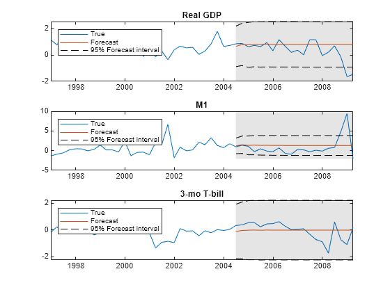
extractMSE = @(x)diag(x)';
MSE = cellfun(extractMSE,FYCov2,UniformOutput=false);
SE = sqrt(cell2mat(MSE));

YFI = zeros(fh,EstMdl2.NumSeries,2);
YFI(:,:,1) = FY2 - 2*SE;
YFI(:,:,2) = FY2 + 2*SE;
This plot shows the predictions of the best fitting model in the shaded region to the right.
figure
tiledlayout(3,1)
for j = 1:EstMdl2.NumSeries
    nexttile
    h1 = plot(Data.Time((end-49):end),Data{(end-49):end,j});
    hold on
    h2 = plot(Data.Time(idxF),FY2(:,j));
    h3 = plot(Data.Time(idxF),YFI(:,j,1),"k--");
    plot(Data.Time(idxF),YFI(:,j,2),"k--");
    title(EstMdl2.SeriesNames{j})
    h = gca;
    fill([Data.Time(idxF(1)) h.XLim([2 2]) Data.Time(idxF(1))], ...
        h.YLim([1 1 2 2]),"k",FaceAlpha=0.1,EdgeColor="none");
    legend([h1 h2 h3],"True","Forecast","95% Forecast interval", ...
        Location="northwest")
    hold off
end
Calculate the sum-of-squares error between the predictions and the data.
Error1 = Data{idxF,:} - FY1;
Error2 = Data{idxF,:} - FY2;
Error3 = Data{idxF,:} - FY3;
Error4 = Data{idxF,:} - FY4;

SSerror1 = Error1(:)' * Error1(:);
SSerror2 = Error2(:)' * Error2(:);
SSerror3 = Error3(:)' * Error3(:);
SSerror4 = Error4(:)' * Error4(:);
figure
bar([SSerror1 SSerror2 SSerror3 SSerror4],.5)
ylabel("Sum of squared errors")
set(gca,XTickLabel=["AR2 diag" "AR2 full" "AR4 diag" "AR4 full"])
title("Forecast Sum of Squared Errors")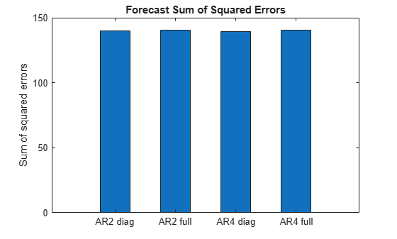
The predictive performances of the four models are similar.
The full AR(2) model seems to be the best and most parsimonious fit. Its model parameters are as follows.
summarize(EstMdl2)
   AR-Stationary 3-Dimensional VAR(2) Model

    Effective Sample Size: 176
    Number of Estimated Parameters: 21
    LogLikelihood: -698.801
    AIC: 1439.6
    BIC: 1506.18

                     Value       StandardError    TStatistic      PValue
                   __________    _____________    __________    __________

    Constant(1)       0.34832       0.11527          3.0217      0.0025132
    Constant(2)       0.55838        0.1488          3.7526     0.00017502
    Constant(3)      -0.45434       0.15245         -2.9803      0.0028793
    AR{1}(1,1)        0.26252       0.07397          3.5491     0.00038661
    AR{1}(2,1)      -0.029371      0.095485         -0.3076        0.75839
    AR{1}(3,1)        0.22324      0.097824          2.2821       0.022484
    AR{1}(1,2)      -0.074627      0.054476         -1.3699        0.17071
    AR{1}(2,2)         0.2531      0.070321          3.5992     0.00031915
    AR{1}(3,2)      -0.017245      0.072044        -0.23936        0.81082
    AR{1}(1,3)       0.032692      0.056182         0.58189        0.56064
    AR{1}(2,3)       -0.35827      0.072523           -4.94     7.8112e-07
    AR{1}(3,3)       -0.29179        0.0743         -3.9272     8.5943e-05
    AR{2}(1,1)        0.21378      0.071283          2.9991      0.0027081
    AR{2}(2,1)      -0.078493      0.092016        -0.85304        0.39364
    AR{2}(3,1)        0.24919      0.094271          2.6433      0.0082093
    AR{2}(1,2)        0.13137      0.051691          2.5415       0.011038
    AR{2}(2,2)        0.38189      0.066726          5.7233      1.045e-08
    AR{2}(3,2)       0.049403      0.068361         0.72269        0.46987
    AR{2}(1,3)       -0.22794      0.059203           -3.85     0.00011809
    AR{2}(2,3)     -0.0052932      0.076423       -0.069262        0.94478
    AR{2}(3,3)       -0.37109      0.078296         -4.7397     2.1408e-06


   Innovations Covariance Matrix:
    0.5931    0.0611    0.1705
    0.0611    0.9882   -0.1217
    0.1705   -0.1217    1.0372


   Innovations Correlation Matrix:
    1.0000    0.0798    0.2174
    0.0798    1.0000   -0.1202
    0.2174   -0.1202    1.0000
Forecast Observations
You can make predictions or forecasts using the fitted model (EstMdl2) either by:
Calling
forecastand passing the last few rows ofYFSimulating several time series with
simulate
In both cases, transform the forecasts so they are directly comparable to the original time series.
Generate 10 predictions from the fitted model beginning at the latest times using forecast.
[YPred,YCov] = forecast(EstMdl2,10,Data{idxF,:});Transform the predictions by undoing the scaling and differencing applied to the original data. Make sure to insert the last observation at the beginning of the time series before using cumsum to undo the differencing. And, since differencing occurred after taking logarithms, insert the logarithm before using cumsum.
YFirst = DataTimeTable(:,["RGDP" "M1SL" "TB3MS"]);
EndPt = YFirst{end,:};
EndPt(:,1:2) = log(EndPt(:,1:2));
YPred(:,1:2) = YPred(:,1:2)/100;     % Rescale percentage
YPred = [EndPt; YPred];              % Prepare for cumsum
YPred = cumsum(YPred);
YPred(:,1:2) = exp(YPred(:,1:2));
fdates = dateshift(YFirst.Time(end),"end","quarter",0:10); % Insert forecast horizon

figure
tiledlayout(3,1)
for j = 1:EstMdl2.NumSeries
    nexttile
    plot(fdates,YPred(:,j),"--b")
    hold on
    plot(YFirst.Time,YFirst{:,j},"k")
    grid on
    title(EstMdl2.SeriesNames{j})
    h = gca;
    fill([fdates(1) h.XLim([2 2]) fdates(1)],h.YLim([1 1 2 2]),"k", ...
        FaceAlpha=0.1,EdgeColor="none");
    hold off
end
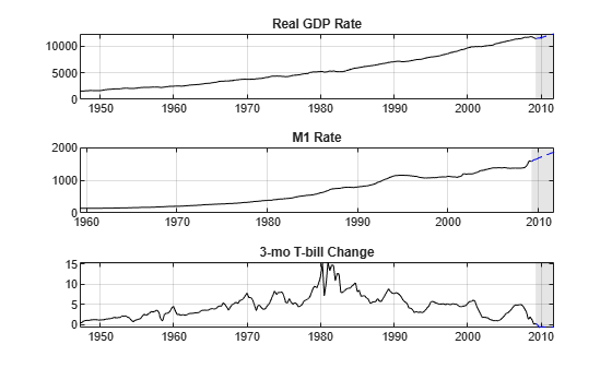
The plots show the extrapolations as blue dashed lines in the light gray forecast horizon, and the original data series in solid black.
Look at the last few years in this plot to get a sense of how the predictions relate to the latest data points.
YLast = YFirst(170:end,:);

figure
tiledlayout(3,1)
for j = 1:EstMdl2.NumSeries
    nexttile
    plot(fdates,YPred(:,j),"b--")
    hold on
    plot(YLast.Time,YLast{:,j},"k")
    grid on
    title(EstMdl2.SeriesNames{j})
    h = gca;
    fill([fdates(1) h.XLim([2 2]) fdates(1)],h.YLim([1 1 2 2]),"k", ...
        FaceAlpha=0.1,EdgeColor="none");
    hold off
end
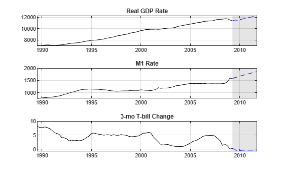
The forecast shows increasing real GDP and M1, and a slight decline in the interest rate. However, the forecast has no error bars.
Alternatively, you can generate 10 predictions from the fitted model beginning at the latest times using simulate. This method simulates 2000 time series times, and then generates the means and standard deviations for each period. The means of the deviates for each period are the predictions for that period.
Simulate a time series from the fitted model beginning at the latest times.
rng(1); % For reproducibility
YSim = simulate(EstMdl2,10,Y0=Data{idxF,:},NumPaths=2000);
Transform the predictions by undoing the scaling and differencing applied to the original data. Make sure to insert the last observation at the beginning of the time series before using cumsum to undo the differencing. And, since differencing occurred after taking logarithms, insert the logarithm before using cumsum.
EndPt = YFirst{end,:};
EndPt(1:2) = log(EndPt(1:2));
YSim(:,1:2,:) = YSim(:,1:2,:)/100;
YSim = [repmat(EndPt,[1,1,2000]);YSim];
YSim(:,1:3,:) = cumsum(YSim(:,1:3,:));
YSim(:,1:2,:) = exp(YSim(:,1:2,:));
Compute the mean and standard deviation of each series, and plot the results. The plot has the mean in black, with a +/- 1 standard deviation in red.
YMean = mean(YSim,3);
YSTD = std(YSim,0,3);

figure
tiledlayout(3,1)
for j = 1:EstMdl2.NumSeries
    nexttile
    plot(fdates,YMean(:,j),"k")
    grid on
    hold on
    plot(YLast.Time(end-10:end),YLast{end-10:end,j},"k")
    plot(fdates,YMean(:,j) + YSTD(:,j),"--r")
    plot(fdates,YMean(:,j) - YSTD(:,j),"--r")
    title(EstMdl2.SeriesNames{j})
    h = gca;
    fill([fdates(1) h.XLim([2 2]) fdates(1)],h.YLim([1 1 2 2]),"k", ...
        FaceAlpha=0.1,EdgeColor="none");
    hold off
end
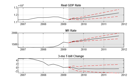
The plots show increasing growth in GDP, moderate to little growth in M1, and uncertainty about the direction of T-bill rates.
See Also
Objects
Functions
estimate|forecast|simulate|lratiotest|aicbic