forecast

Forecast vector autoregression (VAR) model responses

Syntax

Y = forecast(Mdl,numperiods,Y0)

Y = forecast(Mdl,numperiods,Y0,Name=Value)

[Y,YMSE] = forecast(___)

Tbl2 = forecast(Mdl,numperiods,Tbl1)

Tbl2 = forecast(Mdl,numperiods,Tbl1,Name=Value)

[Tbl2,YMSE] = forecast(___)

Tbl2 = forecast(Mdl,numperiods,Tbl1,InSample=InSample,ResponseVariables=ResponseVariables)

Tbl2 = forecast(Mdl,numperiods,Tbl1,InSample=InSample,ResponseVariables=ResponseVariables,Name=Value)

[Tbl2,YMSE] = forecast(___)

Description

Conditional and Unconditional Forecasts for Numeric Arrays

Y = forecast(Mdl,numperiods,Y0) returns a numeric array containing paths of minimum mean squared error (MMSE) multivariate response forecasts Y over a length numperiods forecast horizon, using the fully specified VAR(p) model Mdl. The forecasted responses represent the continuation of the presample data in the numeric array Y0.

Y = forecast(Mdl,numperiods,Y0,Name=Value) uses additional options specified by one or more name-value arguments. forecast returns numeric arrays when all optional input data are numeric arrays. For example, forecast(Mdl,10,Y0,X=Exo) returns a numeric array containing a 10-period forecasted response path from Mdl and the numeric matrix of presample response data Y0, and specifies the numeric matrix of future predictor data for the model regression component in the forecast horizon Exo.

To produce a conditional forecast, specify future response data in a numeric array by using the YF name-value argument.

[Y,YMSE] = forecast(___) also returns the corresponding forecast mean squared error (MSE) matrices YMSE of each forecasted multivariate response using any input argument combination in the previous syntaxes.

Unconditional Forecasts for Tables and Timetables

Tbl2 = forecast(Mdl,numperiods,Tbl1) returns the table or timetable Tbl2 containing the length numperiods paths of multivariate MMSE response variable forecasts, which result from computing unconditional forecasts from the VAR model Mdl. forecast uses the table or timetable of presample data Tbl1 to initialize the response series. (since R2022b)

forecast selects the variables in Mdl.SeriesNames to forecast, or it selects all variables in Tbl1. To select different response variables in Tbl1 to forecast, use the PresampleResponseVariables name-value argument.

Tbl2 = forecast(Mdl,numperiods,Tbl1,Name=Value) uses additional options specified by one or more name-value arguments. For example, forecast(Mdl,10,Tbl1,PresampleResponseVariables=["GDP" "CPI"]) returns a timetable of response variables containing their unconditional forecasts from the VAR model Mdl, initialized by the data in the GDP and CPI variables of the timetable of presample data in Tbl1. (since R2022b)

[Tbl2,YMSE] = forecast(___) also returns the corresponding forecast MSE matrices YMSE of each forecasted multivariate response using any input argument combination in the previous two syntaxes. (since R2022b)

Conditional Forecasts for Tables and Timetables

Tbl2 = forecast(Mdl,numperiods,Tbl1,InSample=InSample,ResponseVariables=ResponseVariables) returns the table or timetable Tbl2 containing the length numperiods paths of multivariate MMSE response variable forecasts and corresponding forecast MSEs, which result from computing conditional forecasts from the VAR model Mdl. forecast uses the table or timetable of presample data Tbl1 to initialize the response series. InSample is a table or timetable of future data in the forecast horizon that forecast uses to compute conditional forecasts and ResponseVariables specifies the response variables in InSample. (since R2022b)

Tbl2 = forecast(Mdl,numperiods,Tbl1,InSample=InSample,ResponseVariables=ResponseVariables,Name=Value) uses additional options specified by one or more name-value arguments. (since R2022b)

[Tbl2,YMSE] = forecast(___) also returns the corresponding forecast MSE matrices YMSE of each forecasted multivariate response using any input argument combination in the previous two syntaxes. (since R2022b)

Examples

Return Matrix of VAR Model Forecasts

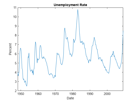
Fit a VAR(4) model to the consumer price index (CPI) and unemployment rate. Then, forecast unconditional MMSE responses from the estimated model. Supply all required data in numeric matrices.

Load the Data_USEconModel data set.

load Data_USEconModel
dts = datetime(dates,ConvertFrom="datenum");

Plot the two series on separate plots.

figure
plot(dts,DataTimeTable.CPIAUCSL);
title("Consumer Price Index")
ylabel("Index")
xlabel("Date")

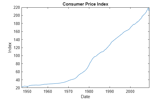
figure
plot(dts,DataTimeTable.UNRATE);
title("Unemployment Rate")
ylabel("Percent")
xlabel("Date")

Stabilize the CPI by converting it to a series of growth rates. Synchronize the two series by removing the first observation from the unemployment rate series.

RCPI = price2ret(DataTimeTable.CPIAUCSL);
UNRATE = DataTimeTable.UNRATE(2:end);
dts = dts(2:end);
EstY = [RCPI UNRATE];

Create a default VAR(4) model by using the shorthand syntax.

Mdl = varm(2,4);

Estimate the model using the entire data set.

EstMdl = estimate(Mdl,EstY);

EstMdl is a fully specified, estimated varm model object.

Forecast responses from the estimated model over a three-year horizon. Specify the entire data set as presample observations.

numperiods = 12;
Y0 = EstY;
Y = forecast(EstMdl,numperiods,Y0);

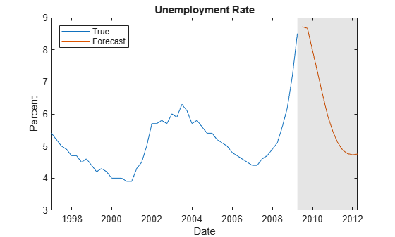
Y is a 12-by-2 matrix of forecasted responses. The first and second columns contain the forecasted CPI growth rate and unemployment rate, respectively.

Plot the forecasted responses and the last 50 true responses.

fh = dateshift(dts(end),"end","quarter",1:numperiods);

figure
h1 = plot(dts((end-49):end),EstY((end-49):end,1));
hold on
h2 = plot(fh,Y(:,1));
title("CPI Growth Rate")
ylabel("Growth Rate")
xlabel("Date")
h = gca;
fill([dts(end) fh([end end]) dts(end)],h.YLim([1 1 2 2]),"k", ...
    FaceAlpha=0.1,EdgeColo="none");
legend([h1 h2],"Data","Forecast")
hold off

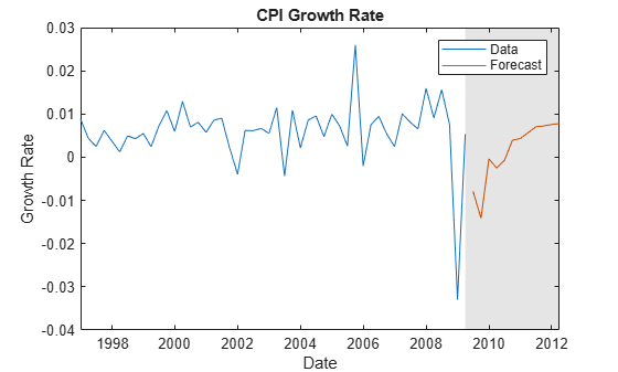
figure
h1 = plot(dts((end-49):end),EstY((end-49):end,2));
hold on
h2 = plot(fh,Y(:,2));
title("Unemployment Rate")
ylabel("Percent")
xlabel("Date")
h = gca;
fill([dts(end) fh([end end]) dts(end)],h.YLim([1 1 2 2]),"k", ...
    FaceAlpha=0.1,EdgeColo="none");
legend([h1 h2],"True","Forecast",Location="northwest")
hold off

Compute Conditional Forecasts from Numeric Matrix of Future Response Data

This example is based on Return Matrix of VAR Model Forecasts. Forecast MMSE responses of the consumer price index (CPI) growth rate four quarters beyond the sampling data, given that the unemployment rate is 8% for each future quarter in the forecast horizon.

Load the Data_USEconModel data set.

load Data_USEconModel
dts = datetime(dates,ConvertFrom="datenum");

Stabilize the CPI by converting it to a series of growth rates. Synchronize the two series by removing the first observation from the unemployment rate series.

RCPI = price2ret(DataTimeTable.CPIAUCSL);
UNRATE = DataTimeTable.UNRATE(2:end);
dts = dts(2:end);
EstY = [RCPI UNRATE];

Create a default VAR(4) model using the shorthand syntax. Estimate the model using the entire data set.

Mdl = varm(2,4);
EstMdl = estimate(Mdl,EstY);

Forecast the CPI growth rate from the estimated model over a one-year horizon, given that the unemployment rate over the next year is 8% each quarter. Create a 2-by-4 matrix CondYF containing the conditions in the forecast horizon, in which the first column (corresponding to RCPI) is composed of NaN values and the second column (corresponding to UNRATE) is completely composed of 8. Supply the future data to forecast and specify the entire data set as presample observations.

numperiods = 4;
Y0 = EstY;
CondYF = NaN(numperiods,Mdl.NumSeries);
CondYF(:,2) = 8;
Y = forecast(EstMdl,numperiods,Y0,YF=CondYF)

Y = 4×2

   -0.0068    8.0000
   -0.0121    8.0000
    0.0006    8.0000
   -0.0045    8.0000

Y is a 4-by-2 matrix of the forecasted CPI growth rate series into the next year, with the unemployment rate fixed at 8%.

Estimate Forecast Intervals

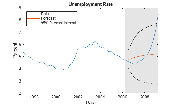
Analyze forecast accuracy using forecast intervals over a three-year horizon. This example follows from Return Matrix of VAR Model Forecasts.

Load the Data_USEconModel data set and preprocess the data.

load Data_USEconModel
dts = datetime(dates,ConvertFrom="datenum");

RCPI = price2ret(DataTimeTable.CPIAUCSL);
UNRATE = DataTimeTable.UNRATE(2:end);
D = [RCPI UNRATE];

Estimate a VAR(4) model of the two response series. Reserve the last three years of data.

bfh = dts(end) - years(3);
estIdx = dts < bfh;
Mdl = varm(2,4);
EstY = D(estIdx,:);
EstMdl = estimate(Mdl,EstY);

Forecast responses from the estimated model over a three-year horizon. Specify the entire data set as presample observations. Return the MSE of the forecasts.

numperiods = 12;
[Y,YMSE] = forecast(EstMdl,numperiods,EstY);

Y is a 12-by-2 matrix of forecasted responses. YMSE is a 12-by-1 cell vector of corresponding MSE matrices.

Extract the main diagonal elements from the matrices in each cell of YMSE. Apply the square root of the result to obtain standard errors.

extractMSE = @(x)diag(x)';
MSE = cellfun(extractMSE,YMSE,UniformOutput=false);
SE = sqrt(cell2mat(MSE));

Estimate approximate 95% forecast intervals for each response series.

YFI = zeros(numperiods,Mdl.NumSeries,2);

YFI(:,:,1) = Y - 2*SE;
YFI(:,:,2) = Y + 2*SE;

Plot the forecasted responses and the last 50 true responses.

figure
h1 = plot(dts((end-49):end),RCPI((end-49):end));
hold on;
h2 = plot(dts(~estIdx),Y(:,1));
h3 = plot(dts(~estIdx),YFI(:,1,1),"k--");
plot(dts(~estIdx),YFI(:,1,2),"k--");
title("CPI Growth Rate")
ylabel("Growth Rate")
xlabel("Date")
h = gca;
fill([bfh h.XLim([2 2]) bfh],h.YLim([1 1 2 2]),"k", ...
    FaceAlpha=0.1,EdgeColor="none");
legend([h1 h2 h3],"Data","Forecast","95% forecast interval", ...
    Location="northwest")
hold off

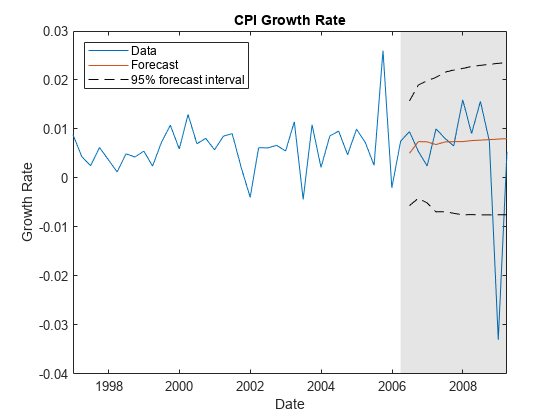
figure
h1 = plot(dts((end-49):end),UNRATE((end-49):end));
hold on;
h2 = plot(dts(~estIdx),Y(:,2));
h3 = plot(dts(~estIdx),YFI(:,2,1),"k--");
plot(dts(~estIdx),YFI(:,2,2),"k--");
title('Unemployment Rate')
ylabel('Percent')
xlabel('Date')
h = gca;
fill([bfh h.XLim([2 2]) bfh],h.YLim([1 1 2 2]),"k", ...
    FaceAlpha=0.1,EdgeColor="none");
legend([h1 h2 h3],"Data","Forecast","95% forecast interval", ...
    Location="northwest")
hold off

Return Timetable of Forecasts and Array of Forecast MSEs

Since R2022b

Fit a VAR(4) model to the consumer price index (CPI) and unemployment rate. Then, forecast unconditional MMSE responses from the estimated model. Supply all required data in timetables. This example is based on Return Response Series in Matrix from Unconditional Simulation.

Load and Preprocess Data

Load the Data_USEconModel data set. Compute the CPI growth rate. Because the growth rate calculation consumes the earliest observation, include the rate variable in the timetable by prepending the series with NaN.

load Data_USEconModel
DataTimeTable.RCPI = [NaN; price2ret(DataTimeTable.CPIAUCSL)];

Prepare Timetable for Estimation

When you plan to supply a timetable directly to estimate, you must ensure it has all the following characteristics:

• All selected response variables are numeric and do not contain any missing values.

• The timestamps in the Time variable are regular, and they are ascending or descending.

Remove all missing values from the table, relative to the CPI rate (RCPI) and unemployment rate (UNRATE) series.

varnames = ["RCPI" "UNRATE"];
DTT = rmmissing(DataTimeTable,DataVariables=varnames);
numobs = height(DTT)

numobs = 
245

rmmissing removes the four initial missing observations from the DataTimeTable to create a sub-table DTT. The variables RCPI and UNRATE of DTT do not have any missing observations.

Determine whether the sampling timestamps have a regular frequency and are sorted.

areTimestampsRegular = isregular(DTT,"quarters")

areTimestampsRegular = logical
   0

areTimestampsSorted = issorted(DTT.Time)

areTimestampsSorted = logical
   1

areTimestampsRegular = 0 indicates that the timestamps of DTT are irregular. areTimestampsSorted = 1 indicates that the timestamps are sorted. Macroeconomic series in this example are timestamped at the end of the month. This quality induces an irregularly measured series.

Remedy the time irregularity by shifting all dates to the first day of the quarter.

dt = DTT.Time;
dt = dateshift(dt,"start","quarter");
DTT.Time = dt;
areTimestampsRegular = isregular(DTT,"quarters")

areTimestampsRegular = logical
   1

DTT is regular with respect to time.

Create Model Template for Estimation

Create a default VAR(4) model by using the shorthand syntax. Specify the response variable names.

Mdl = varm(2,4);
Mdl.SeriesNames = varnames;

Fit Model to Data

Estimate the model. Pass the entire timetable DTT. By default, estimate selects the response variables in Mdl.SeriesNames to fit to the model. Alternatively, you can use the ResponseVariables name-value argument.

EstMdl = estimate(Mdl,DTT);

Forecast Responses and Compute Forecast MSEs

Forecast responses from the estimated model over a three-year horizon. Specify the entire data set DTT as a presample observations.

numperiods = 12;
[Tbl2,YMSE] = forecast(EstMdl,numperiods,DTT);
Tbl2

Tbl2=12×2 timetable
    Time     RCPI_Responses    UNRATE_Responses
    _____    ______________    ________________

    Q2-09      -0.0078947           8.7104     
    Q3-09       -0.014099           8.6682     
    Q4-09     -0.00036087           7.9762     
    Q1-10      -0.0025178           7.3152     
    Q2-10     -0.00074203           6.6233     
    Q3-10       0.0039157           5.9685     
    Q4-10       0.0043404           5.4787     
    Q1-11       0.0056518           5.1184     
    Q2-11       0.0070472           4.8808     
    Q3-11        0.007241           4.7632     
    Q4-11       0.0075783            4.728     
    Q1-12       0.0077906           4.7519     

YMSE

YMSE=12×1 cell array
    {2×2 double}
    {2×2 double}
    {2×2 double}
    {2×2 double}
    {2×2 double}
    {2×2 double}
    {2×2 double}
    {2×2 double}
    {2×2 double}
    {2×2 double}
    {2×2 double}
    {2×2 double}

Tbl2 is a 12-by-2 timetable of forecasted CPI growth and unemployment rates. Forecast variable names are appended with _Responses, for example, RCPI_Responses contains the forecasts of RCPI. The timestamps of Tbl2 follow directly from the timestamps of DTT, and they have the same sampling frequency.

YMSE is a 12-by-1 cell vector of corresponding 2-by-2 forecast MSE matrices for each period in the forecast horizon. For example, the forecast covariance between each response series in period 6 for the forecast horizon (off diagonal of YMSE{6}) is –0.0025.

Forecast VARX(4) Model

Since R2022b

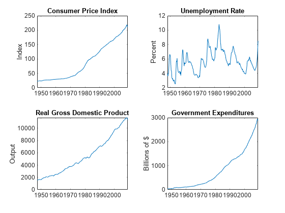
Estimate a four-degree vector autoregression model including exogenous predictors (VARX(4)) of the consumer price index (CPI), the unemployment rate, and the gross domestic product (GDP). Include a linear regression component containing the current quarter and the last four quarters of government consumption expenditures and investment (GCE). Forecast a response path from the estimated model.

Load the Data_USEconModel data set. Compute the real GDP.

load Data_USEconModel
DataTimeTable.RGDP = DataTimeTable.GDP./DataTimeTable.GDPDEF*100;

Plot all variables on separate plots.

figure
tiledlayout(2,2)
nexttile
plot(DataTimeTable.Time,DataTimeTable.CPIAUCSL);
ylabel("Index")
title("Consumer Price Index")
nexttile
plot(DataTimeTable.Time,DataTimeTable.UNRATE);
ylabel("Percent")
title("Unemployment Rate")
nexttile
plot(DataTimeTable.Time,DataTimeTable.RGDP);
ylabel("Output")
title("Real Gross Domestic Product")
nexttile
plot(DataTimeTable.Time,DataTimeTable.GCE);
ylabel("Billions of $")
title("Government Expenditures")

Stabilize the CPI, GDP, and GCE by converting each to a series of growth rates. Synchronize the unemployment rate series with the others by removing its first observation.

varnames = ["CPIAUCSL" "RGDP" "GCE"];
DTT = varfun(@price2ret,DataTimeTable,InputVariables=varnames);
DTT.Properties.VariableNames = varnames;
DTT.UNRATE = DataTimeTable.UNRATE(2:end);

Make the time base regular.

dt = DTT.Time;
dt = dateshift(dt,"start","quarter");
DTT.Time = dt;

Expand the GCE rate series to a matrix that includes the first lagged series through the fourth lag series.

RGCELags = lagmatrix(DTT,1:4,DataVariables="GCE");
DTT = [DTT RGCELags];
DTT = rmmissing(DTT);

Create separate presample and estimation sample data sets. The presample contains the earliest p = 4 observations, and the estimation sample contains the rest of the data.

p = 4;
PS = DTT(1:p,:);
InSample = DTT((p+1):end,:);
respnames = ["CPIAUCSL" "UNRATE" "RGDP"];
idx = endsWith(InSample.Properties.VariableNames,"GCE");
prednames = InSample.Properties.VariableNames(idx);

Create a default VAR(4) model by using the shorthand syntax. Specify the response variable names.

Mdl = varm(3,p);
Mdl.SeriesNames = respnames;

Estimate the model using all but the last three years of data. Specify the GCE matrix as data for the regression component.

bfh = DTT.Time(end) - years(3);
estIdx = DTT.Time < bfh;
EstMdl = estimate(Mdl,DTT(estIdx,:),ResponseVariables=respnames, ...
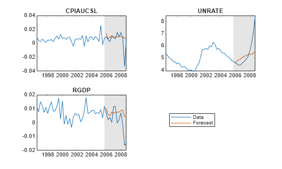
    PredictorVariables=prednames);

Forecast a path of quarterly responses three years into the future.

numperiods = 12;
Tbl1 = DTT(estIdx,:);
Tbl2 = forecast(EstMdl,numperiods,Tbl1,InSample=DTT(~estIdx,:), ...
    PredictorVariables=prednames);

Tbl1 is a 12-by-3 timetable of forecasted responses. Variables names correspond to the response variable names in respnames appended with _Responses.

Plot the forecasted responses and the last 50 true responses.

figure
tiledlayout(2,2)
for j = 1:Mdl.NumSeries
    nexttile
    h1 = plot(DTT.Time((end-49):end),DTT{(end-49):end,respnames(j)});
    hold on
    h2 = plot(DTT.Time(~estIdx),Tbl2{:,respnames(j)+"_Responses"});
    title(respnames(j))
    h = gca;
    fill([bfh h.XLim([2 2]) bfh],h.YLim([1 1 2 2]),"k", ...
        FaceAlpha=0.1,EdgeColor="none");
    hold off
end
hl = legend([h1 h2],["Data" "Forecast"]);
hl.Position = [0.6 0.25 hl.Position(3:4)];

Return Timetable of Conditional Forecasts

Since R2022b

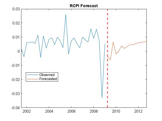
Compute conditional forecasts of the VAR model in Return Timetable of Responses and Innovations from Unconditional Simulation, in which economists hypothesize that the unemployment rate is 6% for 15 quarters after the end of the sample (from Q2 of 2009 through Q4 of 2012).

Load and Preprocess Data

Load the Data_USEconModel data set. Compute the CPI growth rate. Because the growth rate calculation consumes the earliest observation, include the rate variable in the timetable by prepending the series with NaN.

load Data_USEconModel
DataTimeTable.RCPI = [NaN; price2ret(DataTimeTable.CPIAUCSL)];

Prepare Timetable for Estimation

Remove all missing values from the table, relative to the CPI rate (RCPI) and unemployment rate (UNRATE) series.

varnames = ["RCPI" "UNRATE"];
DTT = rmmissing(DataTimeTable,DataVariables=varnames);

Remedy the time irregularity by shifting all dates to the first day of the quarter.

dt = DTT.Time;
dt = dateshift(dt,"start","quarter");
DTT.Time = dt;

Create Model Template for Estimation

Create a default VAR(4) model using the shorthand syntax. Specify the response variable names.

p = 4;
Mdl = varm(2,p);
Mdl.SeriesNames = varnames;

Fit Model to Data

Estimate the model. Pass the entire timetable DTT. By default, estimate selects the response variables in Mdl.SeriesNames to fit to the model. Alternatively, you can use the ResponseVariables name-value argument.

EstMdl = estimate(Mdl,DTT);

Prepare for Conditional Forecast of Estimated Model

Suppose economists hypothesize that the unemployment rate will be at 6% for the next 15 quarters.

Create a timetable with the following qualities:

• The timestamps are regular with respect to the estimation sample timestamps and they are ordered from Q2 of 2009 through Q4 of 2012.

• The variable RCPI (and, consequently, all other variables in DTT) is a 15-by-1 vector of NaN values.

• The variable UNRATE is a 15-by-1 vector, where each element is 6.

numperiods = 15;
fhdt = DTT.Time(end) + calquarters(1:numperiods);
DTTCondF = retime(DTT,fhdt,"fillwithmissing");
DTTCondF.UNRATE = ones(numperiods,1)*6;

DTTCondF is a 15-by-15 timetable that follows directly, in time, from DTT, and both timetables have the same variables. All variables in DTTCondF contain NaN values, except for UNRATE, which is a vector composed of the value 6.

Compute Conditional Forecast of Estimated Model

Forecast the CPI growth rate given the hypothesis by supplying the conditioning data DTTCondF and specifying the response variable names. Supply the estimation sample as a presample to initialize the model.

rng(1) % For reproducibility
Tbl2 = forecast(EstMdl,numperiods,DTT,InSample=DTTCondF, ...
    ResponseVariables=EstMdl.SeriesNames);
size(Tbl2)

ans = 1×2

    15    17

idx = endsWith(Tbl2.Properties.VariableNames,"_Responses");
head(Tbl2(:,idx))

    Time     RCPI_Responses    UNRATE_Responses
    _____    ______________    ________________

    Q2-09      -0.0035362             6        
    Q3-09      -0.0061302             6        
    Q4-09       0.0066157             6        
    Q1-10      -0.0018704             6        
    Q2-10      3.7558e-05             6        
    Q3-10        0.003859             6        
    Q4-10        0.002009             6        
    Q1-11       0.0033291             6        

Tbl2 is a 15-by-17 timetable of all variables in DTTCondF and the RCPI forecasts given UNRATE is 6% for the next 15 quarters. RCPI_Responses contains the forecast path. UNRATE_Responses is a vector composed of the value 6. All other variables in Tbl2 are the variables and their values in DTTCondF.

Plot the CPI growth rate forecast with the final few values of the estimation sample data.

figure
h1 = plot(DTT.Time((end-30):end),DTT.RCPI((end-30):end));
hold on
h2 = plot(Tbl2.Time,Tbl2.RCPI_Responses);
xline(Tbl2.Time(1),"r--",LineWidth=2)
hold off
title("RCPI Forecast")
legend([h1 h2(1)],["Observed" "Forecasted"], ...
    Location="best")

Return Multiple Conditional Forecast Paths

Since R2022b

Compute conditional forecasts of the VAR model in Return Timetable of Responses and Innovations from Unconditional Simulation, in which economists make several hypotheses on the value of the unemployment rate at a forecast horizon of one year.

Load the Data_USEconModel data set. Preprocess the response variables.

load Data_USEconModel
DataTimeTable.RCPI = [NaN; price2ret(DataTimeTable.CPIAUCSL)];

Prepare the timetable for estimation.

varnames = ["RCPI" "UNRATE"];
DTT = rmmissing(DataTimeTable,DataVariables=varnames);
dt = DTT.Time;
dt = dateshift(dt,"start","quarter");
DTT.Time = dt;

Estimate the VAR(4) model.

p = 4;
Mdl = varm(2,p);
Mdl.SeriesNames = varnames;
EstMdl = estimate(Mdl,DTT);

Consider generating several forecast paths of the CPI growth rate assuming the unemployment rate is 1%, 4%, 5%, 8%, and 10% percent throughout the forecast horizon.

Create a timetable with the following qualities:

• The timestamps are regular with respect to the estimation sample timestamps and they are ordered from Q2 of 2009 through Q1 of 2010.

• The variable UNRATE is a 4-by-5 matrix, where each column is composed of each of the assumptions on the value of the unemployment rate in the forecast horizon; the elements of the first column are 1, elements of the second column are 4, and so on.

• The variable RCPI is a 4-by-5 matrix of NaN values to be filled with forecasted paths.

• All other variables are NaN-valued vectors.

numperiods = 4;
fhdt = DTT.Time(end) + calquarters(1:numperiods);
DTTCondF = retime(DTT,fhdt,"fillwithmissing");
DTTCondF.UNRATE = ones(numperiods,1)*[1 4 5 8 10];
DTTCondF.RCPI = nan(numperiods,width(DTTCondF.UNRATE));

DTTCondF is a 4-by-15 timetable that follows directly, in time, from DTT, and both timetables have the same variables. All variables in DTTCondF contain NaN values, except for UNRATE, which is a 4-by-5 matrix of the hypothesized values of the unemployment rate in the forecast horizon.

Forecast the CPI growth rate given the hypotheses by supplying the conditioning data DTTCondF and specifying the response variable names. Supply the estimation sample as a presample to initialize the model. Return the forecast MSE matrices.

rng(1) % For reproducibility
[Tbl2,YMSE] = forecast(EstMdl,numperiods,DTT,InSample=DTTCondF, ...
    ResponseVariables=EstMdl.SeriesNames);
size(Tbl2)

ans = 1×2

     4    17

idx = endsWith(Tbl2.Properties.VariableNames,"_Responses");
head(Tbl2(:,idx))

    Time                                RCPI_Responses                                    UNRATE_Responses     
    _____    _____________________________________________________________________    _________________________

    Q2-09    0.0045044    -0.00031993      -0.001928     -0.0067524     -0.0099686    1     4     5     8    10
    Q3-09    0.0087271    -0.00018729     -0.0031588      -0.012073      -0.018016    1     4     5     8    10
    Q4-09     0.021614       0.012615      0.0096155     0.00061625     -0.0053833    1     4     5     8    10
    Q1-10    0.0045863     0.00071227    -0.00057906     -0.0044531     -0.0070357    1     4     5     8    10

YMSE

YMSE=4×1 cell array
    {2×2 double}
    {2×2 double}
    {2×2 double}
    {2×2 double}

Tbl2 is a 4-by-17 timetable of all variables in DTTCondF. The RCPI forecasts, stored in the variable RCPI_Responses, is a 4-by-5 matrix of five forecast paths. Each path uses the corresponding assumption about the value of unemployment rate in UNRATE_Responses.

YMSE is a 4-by-1 cell vector of forecast MSE matrices for each period in the forecast horizon. The MSE matrices apply to each forecast path, and all elements of each matrix corresponding to the conditioning variable are 0.

Input Arguments

Mdl — VAR model

varm model object

VAR model, specified as a varm model object created by varm or estimate. Mdl must be fully specified.

numperiods — Forecast horizon

positive integer

Forecast horizon, or the number of time points in the forecast period, specified as a positive integer.

Data Types: double

Y0 — Presample response data

numeric matrix | numeric array

Presample response data that provides initial values for the forecasts, specified as a numpreobs-by-numseries numeric matrix or a numpreobs-by-numseries-by-numprepaths numeric array. Use Y0 only when you supply optional data inputs as numeric arrays.

numpreobs is the number of presample observations. numseries is the number of response series (Mdl.NumSeries). numprepaths is the number of presample response paths.

Each row is a presample observation, and measurements in each row, among all pages, occur simultaneously. The last row contains the latest presample observation. Y0 must have at least Mdl.P rows. If you supply more rows than necessary, forecast uses the latest Mdl.P observations only.

Each column corresponds to the response series name in Mdl.SeriesNames.

Pages correspond to separate, independent paths.

• If you compute unconditional forecasts (that is, you do not specify the YF name-value argument), forecast initializes each forecasted path (page) using the corresponding page of Y0. Therefore, the output argument Y has numpaths = numprepaths pages.

• If you compute conditional forecasts by specifying future response data in YF: forecast takes one of these actions:

  • If Y0 is a matrix, forecast initializes each response path (page) in YF using the corresponding presample response in Y0. Therefore, numpaths is the number of paths in YF, and all paths in the output argument Y derive from common initial conditions.

  • If YF is a matrix, forecast generates numprepaths forecast paths, initialized by each presample response path in Y0, but the future response data, from which to condition the forecasts, is the same among all paths. Therefore, numprepaths is the number of paths in the output argument Y, and all paths evolve from possibly different initial conditions.

  • Otherwise, numpaths is the minimum between numprepaths and the number of pages in YF, and forecast applies Y0(:,:,j) to initialize forecasting path j, for j = 1,…,numpaths.

Data Types: double

Tbl1 — Presample data

table | timetable

Since R2022b

Presample response data that provides initial values for the forecasts, specified as a table or timetable with numprevars variables and numpreobs rows. forecast returns the forecasted response variable in the output table or timetable Tbl2, which is commensurate with Tbl1.

Each row is a presample observation, and measurements in each row, among all paths, occur simultaneously. numpreobs must be at least Mdl.P. If you supply more rows than necessary, forecast uses the latest Mdl.P observations only.

Each selected response variable is a numpreobs-by-numprepaths numeric matrix. You can optionally specify numseries response variables by using the PresampleResponseVariables name-value argument.

Paths (columns) within a particular response variable are independent, but path j of all variables correspond, for j = 1,…,numprepaths. The following conditions apply:

• If you compute unconditional forecasts (that is, you do not specify the InSample and ResponseVariables name-value arguments), forecast initializes each forecasted path per selected response variable using the corresponding path in Tbl1. Therefore, each forecasted response variable in the output argument Tbl2 is a numperiods-by-numprepaths matrix.

• If you compute conditional forecasts by specifying future response data in InSample and corresponding response variables from the data by using ResponseVariables, forecast takes one of these actions:

  • If the selected presample response variables are vectors, forecast initializes each forecast path (column) of the selected response variables in InSample by using the corresponding presample variable in Tbl1. Therefore, all paths in the forecasted response variables evolve from common initial conditions.

  • If the selected response variables in InSample are vectors, forecast generates numprepaths forecast paths, initialized by the paths of each selected presample response variable in Tbl1, but the future response data, from which to condition the forecasts, is the same among all paths. Therefore, numpaths = numprepaths is the number of paths in all forecasted response variables, and all paths evolve from possibly different initial conditions.

  • Otherwise, numpaths is the minimum between numprepaths and the number of paths in each selected response variable in InSample. For each selected presample and future sample response variable ResponseK and each path j = 1,…,numpaths, forecast applies Tbl1.ResponseK(:,j) to initialize the conditional forecast for the response data in Tbl2.ResponseK(:,j).

If Tbl1 is a timetable, all the following conditions must be true:

• Tbl1 must represent a sample with a regular datetime time step (see isregular).

• The inputs InSample and Tbl1 must be consistent in time such that Tbl1 immediately precedes InSample with respect to the sampling frequency and order.

• The datetime vector of sample timestamps Tbl1.Time must be ascending or descending.

If Tbl1 is a table, the last row contains the latest presample observation.

InSample — Future time series response or predictor data

table | timetable

Since R2022b

Future time series response or predictor data, specified as a table or timetable. InSample contains numvars variables, including numseries response variables y_t or numpreds predictor variables x_t for the model regression component. You can specify InSample only when you specify Tbl1.

Use InSample in the following situations:

• Perform conditional simulation. You must also supply the response variable names to select response data in InSample by using the ResponseVariables name-value argument.

• Supply future predictor data for either unconditional or conditional simulation. To supply predictor data, you must specify predictor variable names in InSample by using the PredictorVariables name-value argument. Otherwise, forecast ignores the model regression component.

Each row corresponds to an observation in the forecast horizon, the first row is the earliest observation, and measurements in each row, among all paths, occur simultaneously. Specifically, row j of variable VariableK (InSample.VariableK(j,:)) contains observations j periods into the future, or the j-period-ahead forecasts. InSample must have at least numperiods rows to cover the forecast horizon. If you supply more rows than necessary, forecast uses only the first numperiods rows.

Each selected response variable is a numeric matrix. For each selected response variable K, columns are separate, independent paths. Specifically, path j of response variable ResponseK captures the state, or knowledge, of ResponseK as it evolves from the presample past (for example, Tbl1.ResponseK) into the future. For each selected response variable ResponseK:

• If the selected presample response variables in Tbl1 are vectors, forecast initializes each forecast path (column) of the selected response variables in InSample by using the corresponding presample variable in Tbl1. Therefore, all paths in the forecasted response variables of the output Tbl2 evolve from common initial conditions.

• If the selected response variables in InSample are vectors, forecast generates numprepaths forecast paths, initialized by the paths of each selected presample response variable in Tbl1, but the future response data, from which to condition the forecasts, is the same among all paths. Therefore, numpaths = numprepaths is the number of paths in all forecasted response variables, and all paths evolve from possibly different initial conditions.

• Otherwise, numpaths is the minimum between numprepaths and the number of paths in each selected response variable in InSample. For each selected presample and future sample response variable ResponseK and each path j = 1,…,numpaths, forecast applies Tbl1.ResponseK(:,j) to initialize the conditional forecast for the response data in Tbl2.ResponseK(:,j).

Each predictor variable is a numeric vector. All predictor variables are present in the regression component of each response equation and apply to all response paths.

If InSample is a timetable, the following conditions apply:

• InSample must represent a sample with a regular datetime time step (see isregular).

• The datetime vector InSample.Time must be ascending or descending.

• Tbl1 must immediately precede InSample, with respect to the sampling frequency.

If InSample is a table, the last row contains the latest observation.

Elements of the response variables of InSample can be numeric scalars or missing values (indicated by NaN values). forecast treats numeric scalars as deterministic future responses that are known in advance, for example, set by policy. forecast forecasts responses for corresponding NaN values conditional on the known values. Elements of selected predictor variables must be numeric scalars.

By default, forecast computes conventional MMSE forecasts and forecast MSEs without a regression component in the model (each selected response variable is a numperiods-by-numprepaths matrix composed of NaN values indicating a complete lack of knowledge of the future state of the responses in the forecast horizon).

For more details, see Algorithms.

Example: Consider forecasting one path from a model composed of two response series, GDP and CPI, three periods into the future. Suppose that you have prior knowledge about some of the future values of the responses, and you want to forecast the unknown responses conditional on your knowledge. Specify InSample as a matrix containing the values that you know, and use NaN for values you do not know but want to forecast. For example, InSample=array2table([2 NaN; 0.1 NaN; NaN NaN],VariableNames=["GDP" "CPI"]) specifies that you have no knowledge of the future values of CPI, but you know that GDP is 2, 0.1, and unknown in periods 1, 2, and 3, respectively, in the forecast horizon.

ResponseVariables — Variables to select from InSample to treat as response variables y_t

string vector | cell vector of character vectors | vector of integers | logical vector

Since R2022b

Variables to select from InSample to treat as response variables y_t, specified as one of the following data types:

• String vector or cell vector of character vectors containing numseries variable names in InSample.Properties.VariableNames

• A length numseries vector of unique indices (integers) of variables to select from InSample.Properties.VariableNames

• A length numvars logical vector, where ResponseVariables(j) = true selects variable j from InSample.Properties.VariableNames, and sum(ResponseVariables) is numseries

The selected variables must be numeric vectors (single path) or matrices (columns represent multiple independent paths) of the same width.

To compute conditional forecasts, you must specify ResponseVariables to select the response variables in InSample for the conditioning data. ResponseVariables applies only when you specify InSample.

By default, forecast computes conventional MMSE forecasts and forecast MSEs.

Example: ResponseVariables=["GDP" "CPI"]

Example: ResponseVariables=[true false true false] or ResponseVariable=[1 3] selects the first and third table variables as the response variables.

Data Types: double | logical | char | cell | string

Name-Value Arguments

Specify optional pairs of arguments as Name1=Value1,...,NameN=ValueN, where Name is the argument name and Value is the corresponding value. Name-value arguments must appear after other arguments, but the order of the pairs does not matter.

Before R2021a, use commas to separate each name and value, and enclose Name in quotes.

Example: forecast(Mdl,10,Y0,X=Exo) returns a numeric array containing a 10-period forecasted response path from Mdl and the numeric matrix of presample response data Y0, and specifies the numeric matrix of future predictor data for the model regression component in the forecast horizon Exo.

PresampleResponseVariables — Variables to select from Tbl1 to use for presample response data

string vector | cell vector of character vectors | vector of integers | logical vector

Since R2022b

Variables to select from Tbl1 to use for presample data, specified as one of the following data types:

• String vector or cell vector of character vectors containing numseries variable names in Tbl1.Properties.VariableNames

• A length numseries vector of unique indices (integers) of variables to select from Tbl1.Properties.VariableNames

• A length numprevars logical vector, where PresampleResponseVariables(j) = true selects variable j from Tbl1.Properties.VariableNames, and sum(PresampleResponseVariables) is numseries

The selected variables must be numeric vectors and cannot contain missing values (NaN).

PresampleResponseNames does not need to contain the same names as in Mdl.SeriesNames; forecast uses the data in selected variable PresampleResponseVariables(j) as a presample for Mdl.SeriesNames(j).

If the number of variables in Tbl1 matches Mdl.NumSeries, the default specifies all variables in Tbl1. If the number of variables in Tbl1 exceeds Mdl.NumSeries, the default matches variables in Tbl1 to names in Mdl.SeriesNames.

Example: PresampleResponseVariables=["GDP" "CPI"]

Example: PresampleResponseVariables=[true false true false] or PresampleResponseVariable=[1 3] selects the first and third table variables for presample data.

Data Types: double | logical | char | cell | string

X — Forecasted time series of predictor data x_t

numeric matrix

Forecasted time series of predictor data x_t to include in the model regression component, specified as a numeric matrix containing numpreds columns. Use X only when you supply Y0.

numpreds is the number of predictor variables (size(Mdl.Beta,2)).

Each row corresponds to an observation in the forecast horizon, and measurements in each row occur simultaneously. Specifically, row j (X(j,:)) contains the predictor observations j periods into the future, or the j-period-ahead forecasts. X must have at least numperiods rows. If you supply more rows than necessary, forecast uses only the earliest numperiods observations. The first row contains the earliest observation. forecast does not use the regression component in the presample period.

Each column is an individual predictor variable. All predictor variables are present in the regression component of each response equation.

forecast applies X to each path (page); that is, X represents one path of observed predictors.

To maintain model consistency into the forecast horizon, specify forecasted predictors when Mdl has a regression component.

By default, forecast excludes the regression component, regardless of its presence in Mdl.

Data Types: double

YF — Future multivariate response series data

numeric matrix | numeric array

Future multivariate response series data for conditional forecasting, specified as a numeric matrix or array containing numseries columns. Use YF only when you supply Y0.

Each row corresponds to observations in the forecast horizon, and the first row is the earliest observation. Specifically, row j in sample path k (YF(j,:,k)) contains the responses j periods into the future, or the j-period-ahead forecasts. YF must have at least numperiods rows to cover the forecast horizon. If you supply more rows than necessary, forecast uses only the first numperiods rows.

Each column corresponds to the response variable name in Mdl.SeriesNames.

Each page corresponds to a separate sample path. Specifically, path k (YF(:,:,k)) captures the state, or knowledge, of the response series as they evolve from the presample past (Y0) into the future.

• If YF is a matrix, forecast generates numprepaths forecast paths, initialized by each presample response path in Y0, but the future response data, from which to condition the forecasts, is the same among all paths. Therefore, numprepaths is the number of paths in the output argument Y, and all paths evolve from possibly different initial conditions.

• If Y0 is a matrix, forecast initializes each response path (page) in YF using the corresponding presample response in Y0. Therefore, numpaths is the number of paths in YF, and all paths in the output argument Y derive from common initial conditions.

• Otherwise, numpaths is the minimum between numprepaths and the number of pages in YF, and forecast applies Y0(:,:,j) to initialize forecasting path j, for j = 1,…,numpaths.

Elements of YF can be numeric scalars or missing values (indicated by NaN values). forecast treats numeric scalars as deterministic future responses that are known in advance, for example, set by policy. forecast forecasts responses for corresponding NaN values conditional on the known values.

By default, YF is an array composed of NaN values indicating a complete lack of knowledge of all responses in the forecast horizon. In this case, forecast estimates conventional MMSE forecasts.

For more details, see Algorithms.

Example: Consider forecasting one path from a model composed of four response series three periods into the future. Suppose that you have prior knowledge about some of the future values of the responses, and you want to forecast the unknown responses conditional on your knowledge. Specify YF as a matrix containing the values that you know, and use NaN for values you do not know but want to forecast. For example, YF=[NaN 2 5 NaN; NaN NaN 0.1 NaN; NaN NaN NaN NaN] specifies that you have no knowledge of the future values of the first and fourth response series; you know the value for period 1 in the second response series, but no other value; and you know the values for periods 1 and 2 in the third response series, but not the value for period 3.

Data Types: double

PredictorVariables — Variables to select from InSample to treat as exogenous predictor variables x_t

string vector | cell vector of character vectors | vector of integers | logical vector

Since R2022b

Variables to select from InSample to treat as exogenous predictor variables x_t, specified as one of the following data types:

• String vector or cell vector of character vectors containing numpreds variable names in InSample.Properties.VariableNames

• A length numpreds vector of unique indices (integers) of variables to select from InSample.Properties.VariableNames

• A length numvars logical vector, where PredictorVariables(j) = true selects variable j from InSample.Properties.VariableNames, and sum(PredictorVariables) is numpreds

Regardless, selected predictor variable j corresponds to the coefficients Mdl.Beta(:,j).

PredictorVariables applies only when you specify InSample.

The selected variables must be numeric vectors and cannot contain missing values (NaN).

By default, forecast excludes the regression component, regardless of its presence in Mdl.

Example: PredictorVariables=["M1SL" "TB3MS" "UNRATE"]

Example: PredictorVariables=[true false true false] or PredictorVariable=[1 3] selects the first and third table variables as the response variables.

Data Types: double | logical | char | cell | string

Note

• NaN values in Y0 and X indicate missing values. forecast removes missing values from the data by list-wise deletion. If Y0 is a 3-D array, then forecast performs these steps:

  1. Horizontally concatenate pages to form a numpreobs-by-numpaths*numseries matrix.

  2. Remove any row that contains at least one NaN from the concatenated data.

  In the case of missing observations, the results obtained from multiple paths of Y0 can differ from the results obtained from each path individually.

  For missing values in X, forecast removes the corresponding row from each page of YF. After row removal from X and YF, if the number of rows is less than numperiods, forecast issues an error.

• forecast issues an error when selected response variables from Tbl1 and selected predictor variables from InSample contain any missing values.

Output Arguments

Y — MMSE forecasts of multivariate response series

numeric matrix | numeric array

MMSE forecasts of the multivariate response series, returned as a numobs-by-numseries numeric matrix or a numobs-by-numseries-by-numpaths numeric array. forecast returns Y only when you supply presample data Y0 as a numeric matrix or array.

Y represents the continuation of the presample responses in Y0.

Each row is a time point in the simulation horizon. Specifically, row j contains the j-period-ahead forecasts. Values in a row, among all pages, occur simultaneously. The last row contains the latest forecasted values.

Each column corresponds to the response series name in Mdl.SeriesNames.

Pages correspond to separate, independently forecasted paths.

If you specify future responses for conditional forecasting using the YF name-value argument, the known values in YF appear in the same positions in Y. However, Y contains forecasted values for the missing observations in YF.

Tbl2 — MMSE forecasts of multivariate response series and other variables

table | timetable

Since R2022b

MMSE forecasts of multivariate response series and other variables, returned as a table or timetable, the same data type as Tbl1. forecast returns Tbl2 only when you supply the inputs Tbl1.

Tbl2 contains the following variables:

• The forecasted response paths within the numperiods length forecast horizon of the selected response series y_t. Each forecasted response variable in Tbl2 is a numperiods-by-numpaths numeric matrix, where numpaths depends on the number of response paths in the specified presample or future sample data (see Tbl1 or InSample). Each row corresponds to a time in the forecast horizon and each column corresponds to a separate path. forecast names the forecasted response variable ResponseK ResponseK_Responses. For example, if Mdl.Series(K) is GDP, Tbl2 contains a variable for the corresponding forecasted response with the name GDP_Responses. If you specify ResponseVariables, ResponseK is ResponseVariable(K). Otherwise, ResponseK is PresampleResponseVariable(K).

• If you specify InSample, all specified future response variables.

If Tbl2 is a timetable, the following conditions hold:

• The row order of Tbl2, either ascending or descending, matches the row order of InSample, when you specify it. If you do not specify InSample, the row order of Tbl2 is the same as the row order Tbl1.

• If you specify InSample, row times Tbl2.Time are InSample.Time(1:numperiods). Otherwise, Tbl2.Time(1) is the next time after Tbl1(end) relative to the sampling frequency, and Tbl2.Time(2:numperiods) are the following times relative to the sampling frequency.

YMSE — MSE matrices of forecasted responses

cell vector of numeric matrices

MSE matrices of the forecasted responses, returned as a numperiods-by-1 cell vector of numseries-by-numseries numeric matrices. Cells of YMSE compose a time series of forecast error covariance matrices. Cell j contains the j-period-ahead MSE matrix.

YMSE is identical for all paths.

Because forecast treats predictor variables in X as exogenous and nonstochastic, YMSE reflects the error covariance associated with the autoregressive component of the input model Mdl only.

Algorithms

• forecast estimates unconditional forecasts using the equation

  $${\widehat{y}}_t={\widehat{\Phi }}_1{\widehat{y}}_{t-1}+\mathrm{...}+{\widehat{\Phi }}_p{\widehat{y}}_{t-p}+\widehat{c}+\widehat{\delta }t+\widehat{\beta }{x}_t,$$

  where t = 1,...,numperiods. forecast filters a numperiods-by-numseries matrix of zero-valued innovations through Mdl. forecast uses specified presample innovations (Y0 or Tbl1) wherever necessary.

• forecast estimates conditional forecasts using the Kalman filter.

  1. forecast represents the VAR model Mdl as a state-space model (ssm model object) without observation error.

  2. forecast filters the forecast data YF through the state-space model. At period t in the forecast horizon, any unknown response is

     $${\widehat{y}}_t={\widehat{\Phi }}_1{\widehat{y}}_{t-1}+\mathrm{...}+{\widehat{\Phi }}_p{\widehat{y}}_{t-p}+\widehat{c}+\widehat{\delta }t+\widehat{\beta }{x}_t,$$

     where $${\widehat{y}}_s,$$ s < t, is the filtered estimate of y from period s in the forecast horizon. forecast uses specified presample values in Y0 or Tbl1 for periods before the forecast horizon.

  For more details, see filter and [4], pp. 612 and 615.

• The way forecast determines numpaths, the number of paths (pages) in the output argument Y, or the number of paths (columns) in the forecasted response variables in the output argument Tbl2, depends on the forecast type.

  • If you estimate unconditional forecasts, which means you do not specify the YF name-value argument, or InSample and ResponseVariables name-value arguments, numpaths is the number of paths in the Y0 or Tbl1 input argument.

  • If you estimate conditional forecasts and the presample data Y0 and future sample data YF, or response variables in Tbl1 and InSample have more than one path, numpaths is the fewest number of paths between the presample and future sample response data. Consequently, forecast uses only the first numpaths paths of each response variable for each input.

  • If you estimate conditional forecasts and either Y0 or YF, or response variables in Tbl1 or InSample have one path, numpaths is the number of pages in the array with the most pages. forecast uses the variables with one path to produce each output path.

• forecast sets the time origin of models that include linear time trends t₀ to numpreobs – Mdl.P (after removing missing values), where numpreobs is the number of presample observations. Therefore, the times in the trend component are t = t₀ + 1, t₀ + 2,..., t₀ + numpreobs. This convention is consistent with the default behavior of model estimation in which estimate removes the first Mdl.P responses, reducing the effective sample size. Although forecast explicitly uses the first Mdl.P presample responses in Y0 or Tbl1 to initialize the model, the total number of usable observations determines t₀. An observation in Y0 is usable if it does not contain a NaN.

References

[1] Hamilton, James D. Time Series Analysis. Princeton, NJ: Princeton University Press, 1994.

[2] Johansen, S. Likelihood-Based Inference in Cointegrated Vector Autoregressive Models. Oxford: Oxford University Press, 1995.

[3] Juselius, K. The Cointegrated VAR Model. Oxford: Oxford University Press, 2006.

[4] Lütkepohl, H. New Introduction to Multiple Time Series Analysis. Berlin: Springer, 2005.

Version History

Introduced in R2017a

R2022b: forecast accepts input data in tables and timetables, and return results in tables and timetables

In addition to accepting input data in numeric arrays, forecast accepts input data in tables and timetables. forecast chooses default series on which to operate, but you can use the following name-value arguments to select variables.

• PresampleResponseVariables specifies the response series names in the input presample response data.

• Insample specifies the table or regular timetable of future response and predictor data to compute conditional forecasts.

• ResponseVariables specifies the response series names in InSample.

• PredictorVariables specifies the predictor series in InSample for a model regression component.