Vector Autoregression (VAR) Model Creation
Econometrics Toolbox™ has a class of functions for modeling multivariate time series using a VAR model. The varm function creates a varm object that represents a VAR model. varm properties specify the VAR model structure, including the number of response series (dimensionality), number of autoregressive (AR) lags, and the presence of constant or time trend coefficients in the model.
A varm object can serve as a model template for estimation, in which case you must specify at least the number of response series and the degree of the AR polynomial. Optionally, you can specify values for other parameters (coefficients or innovations covariance matrix) to test hypotheses or economic theory. The estimate object function fits unspecified estimable parameters of the model to specified data, and returns a fully specified varm object. Supply a fully specified model to other varm
object functions for further analysis.
Create VAR Model
You can create a varm object using one of two syntaxes: shorthand or longhand.
The shorthand syntax is suited for the quick creation of a model, usually when the model serves as a template for estimation. The required inputs are the response series dimensionality (numseries) and the degree of the AR polynomial (p). The AR polynomial of the resulting VAR model has nonzero lags 1 through p. For an example, see Create and Adjust VAR Model Using Shorthand Syntax.
The longhand syntax allows for more flexibility in parameter specification than the shorthand syntax. For example, you can specify values of autoregressive coefficient matrices or which lags have nonzero coefficient matrices. Whereas the varm function requires the inputs numseries and p when you use the shorthand syntax, the function must be able to infer these structural characteristics from the values you supply when you use the longhand syntax. In other words, these structural characteristics are not estimable. For an example, see Create and Adjust VAR Model Using Longhand Syntax.
Regardless of syntax, the resulting VAR model is an object. Values of the object properties completely determine the structure of the VAR model. After creating a model, you can display it to verify its structure, and you can change parameter values by adjusting properties using dot notation (see Display and Change Model Objects).
Depending on your analysis goals, you can use one of several methods to create a model using the varm function.
Fully Specified Model Object – Use this method when you know the values of all parameters of your model. That is, you do not plan to fit the model to data.
Model Template for Unrestricted Estimation – Use this method when you know the response dimensionality and the AR polynomial degree, and you want to fit the entire model to data using
estimate.Partially Specified Model Object for Restricted Estimation – Use this method when you know the response dimensionality, AR polynomial degree, as well as some of the parameter values. For example:
You know the values of some AR coefficient matrices or you want to test hypotheses.
You want to exclude some lags from an equation.
You want to exclude some exogenous predictor variables from an equation.
To estimate any unknown parameter values, pass the model object and data to
estimate, which applies equality constraints to all known parameters at their specified values during optimization.Model objects with a regression component for exogenous variables:
If you plan to estimate a multivariate model containing an unrestricted regression component, specify the structure of the model, except the regression component, when you create the model. Then, specify the model and exogenous data (for example, the
Xname-value argument) when you callestimate. Consequently,estimateincludes an appropriately sized regression coefficient matrix in the model, and estimates it.estimateincludes all exogenous variables in the regression component of each response equation by default.If you plan to specify equality constraints in the regression coefficient matrix for estimation, or you want to fully specify the matrix, use the longhand syntax and the
Betaname-value argument to specify the matrix when you create the model. Alternatively, after creating the model, you can specify theBetamodel property by using dot notation. For example, to exclude an exogenous variable from an equation, set the coefficient element corresponding to the variable (column) and equation (row) to0.
varm objects do not store data. Instead, you specify data when you operate on a model by using an object function.
Fully Specified Model Object
If you know the values of all model coefficients and the innovations covariance
matrix, create a model object and specify the parameter values using the longhand
syntax. This table describes the name-value arguments you can pass to the
varm function for known parameter values in a
numseries-dimensional VAR(p) model.
| Name | Value |
|---|---|
Constant
| A |
Lags | A numeric vector of autoregressive polynomial lags. The largest lag determines |
AR | A cell vector of |
Trend | A |
Beta | A |
Covariance | A |
You can also create a model object using the shorthand syntax, and then adjust corresponding property values (except Lags) using dot notation.
The Lags name-value argument allows you to specify which lags
you want to include. For example, to specify AR lags 1 and 3 without lag 2, set
Lags to [1 3]. Although this syntax
specified only two lags, p is 3.
The following example shows how to create a model object when you have known parameters. Consider the VAR(1) model
The independent disturbances εt are distributed as standard 3-D normal random variables.
This code shows how to create a model object using varm.
c  = [0.05; 0; -0.05];
AR = {[.5 0 0;.1 .1 .3;0 .2 .3]};
Covariance = eye(3);
Mdl = varm('Constant',c,'AR',AR,'Covariance',Covariance)
Mdl =
varm with properties:
Description: "AR-Stationary 3-Dimensional VAR(1) Model"
SeriesNames: "Y1" "Y2" "Y3"
NumSeries: 3
P: 1
Constant: [0.05 0 -0.05]'
AR: {3×3 matrix} at lag [1]
Trend: [3×1 vector of zeros]
Beta: [3×0 matrix]
Covariance: [3×3 diagonal matrix]The object display shows property values. The varm function identifies this model as a stationary VAR(1) model with three dimensions, additive constants, no time trend, and no regression component.
Model Template for Unrestricted Estimation
The easiest way to create a multivariate model template for estimation is by using the shorthand syntax. For example, to create a VAR(2) model template for 3 response series by using varm and its shorthand syntax, enter this code.
numseries = 3;
p = 2;
Mdl = varm(numseries,p);
Mdl represents a VAR(2) model containing unknown, estimable parameters, including the constant vector and 3-by-3 lag coefficient matrices from lags 1 through 2.NaN elements in the arrays of the model properties indicate estimable parameters. The Beta property can be a numseries-by-0 array and can be estimable; estimate infers its column dimension from specified exogenous data. When you use the shorthand syntax, varm sets the constant vector, all autoregressive coefficient matrices, and the innovations covariance matrix to appropriately sized arrays of NaNs.
To display the VAR(2) model template Mdl and see which parameters are estimable, enter this code.
Mdl
Mdl =

  varm with properties:

     Description: "3-Dimensional VAR(2) Model"
     SeriesNames: "Y1"  "Y2"  "Y3"
       NumSeries: 3
               P: 2
        Constant: [3×1 vector of NaNs]
              AR: {3×3 matrices of NaNs} at lags [1 2]
           Trend: [3×1 vector of zeros]
            Beta: [3×0 matrix]
      Covariance: [3×3 matrix of NaNs]
Mdl.Trend is a vector of zeros, which indicates that the linear time trend is not a model parameter.To specify model characteristics that are different from the defaults, use the longhand syntax or adjust writable properties of an existing model by using dot notation. For example, this code shows how to create a model containing a linear time-trend term, with an estimable coefficient, by using the longhand syntax.
AR = cell(p,1);
AR(:) = {nan(numseries)}; % varm can infer response dimension and AR degree from AR
MdlLT = varm('AR',AR,'Trend',nan(numseries,1));Mdl to include an estimable linear time-trend term.Mdl.Trend = nan(numseries,1);
estimate fits all unspecified parameters, including the model constant vector, autoregressive coefficient matrices, regression coefficient matrix, linear time-trend vector, and innovations covariance matrix.
Alternatively, you can create an unrestricted VAR model using the Econometric Modeler app. The app treats the model constant and time trend term as unknown and estimable, but it enables you to partially specify elements of the lag coefficient matrices for restricted estimation.
At the command line, open the Econometric Modeler app.
econometricModeler
Alternatively, open the app from the apps gallery (see Econometric Modeler).
In the app, after you load some data, you can see all supported multivariate models by selecting at least two time series variable for the response in the Time Series pane. Then, on the Modeler tab, in the Models section, click the arrow to display the models gallery.
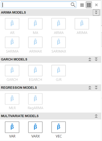
The Multivariate Models section contains all supported
multivariate models. The available VAR models are VAR and VARX. To specify a VAR
model, click VAR. The VAR Model
Parameters dialog box appears.

Adjustable parameters include:
Autoregressive Order (p) – The order of the autoregressive polynomial. Econometric Modeler includes all lags up to the specified value in the model.
Include Constant Term – The inclusion of a model constant, c
Include Trend – The inclusion of a time trend term, δt
As you adjust parameter values, the equation in the Model
Equation section changes to match your specifications. Adjustable
parameters correspond to input and name-value arguments described in the previous
sections and in the varm reference page.
To specify a VARX model, click VARX. The VARX
Model Parameters dialog box appears.
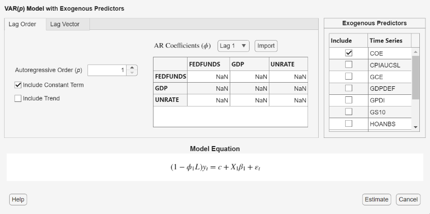
In addition to the adjustable parameters available for VAR models, you can choose which exogenous predictors to include in the model regression component by clicking the Include check box next to the predictor variable in the Exogenous Predictors table.
For more details on specifying models using the app, see Fit Models to Data and Specifying Multivariate Lag Operator Polynomials and Coefficient Constraints Interactively.
Partially Specified Model Object for Restricted Estimation
You can create a model object with some known parameters to test hypotheses about their values. estimate treats the known values as equality constraints during estimation, and fits the remaining unknown parameters to the data. All VAR model coefficients can contain a mix of NaN and valid real numbers, but the innovations covariance matrix must be completely unknown (composed entirely of NaNs) or completely known (a positive definite matrix).
This code shows how to specify the model in Fully Specified Model Object, but the AR parameters have a diagonal autoregressive structure and an unknown innovation covariance matrix. varm infers the dimensionality of the response variable from the parameters c and AR, and infers the degree of the VAR model from AR.
c = [.05; 0; -.05];
AR = {diag(nan(3,1))};
Mdl = varm('Constant',c,'AR',AR)
Mdl.AR{:}
Mdl =
varm with properties:
Description: "3-Dimensional VAR(1) Model"
SeriesNames: "Y1" "Y2" "Y3"
NumSeries: 3
P: 1
Constant: [0.05 0 -0.05]'
AR: {3×3 matrix} at lag [1]
Trend: [3×1 vector of zeros]
Beta: [3×0 matrix]
Covariance: [3×3 matrix of NaNs]
ans =
NaN 0 0
0 NaN 0
0 0 NaNAlternatively, you can create fix elements of the autoregression lag coefficients using the Econometric Modeler app. The app treats all other parameters as unknown and estimable.
At the command line, open the Econometric Modeler app.
econometricModeler
Alternatively, open the app from the apps gallery (see Econometric Modeler).
In the app, after you load some data, select at least two time series variable for
the response in the Time Series pane. Then, on the
Modeler tab, in the Models section,
click the arrow to display the models gallery, and then click
VAR.
In the VAR Model Parameters dialog box, in the AR Coefficients (ϕ) section, use the Lag menu to select a lag to adjust, and then enter values into the table, which represents the corresponding AR coefficient matrix, to specify estimation constraints. NaN values indicate unconstrained elements of the coefficient (estimable).
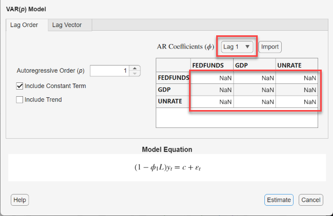
Each row corresponds to the VAR equation of the associated variable (left-hand
side) and each column corresponds to the variable being lagged on the right-hand
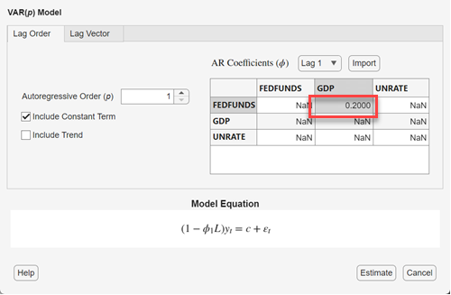
side of the equation. For example, this figure shows how to hold fixed the lag 1
coefficient of GDP in the equation of FEDFUNDS to 0.2:
y1 =
c1 +
ϕ11,1y1,t
– 1 + 0.2y2,t –
1 +
ϕ13,1y3,t
– 1 + εt, where
y1,t is
FEDFUNDS,
y2,t is
GDP, and
y3,t is
UNRATE.
Display and Change Model Objects
Suppose the variable name of a model object is Mdl. After you create Mdl, you can examine it in several ways:
Enter
Mdlat the MATLAB® command line.Double-click the object in the MATLAB Workspace panel.
Enter
Mdl.at the MATLAB command line, wherePropertyNamePropertyName
You can change any writable property of a model object using dot notation:
Mdl.PropertyValue = value;
Display Model Object
Create a VAR(2) model object for three response variables. Use the shorthand syntax.
numseries = 3;
p = 2;
Mdl = varm(numseries,p);
Display the VAR(2) model.
Mdl
Mdl =
  varm with properties:

     Description: "3-Dimensional VAR(2) Model"
     SeriesNames: "Y1"  "Y2"  "Y3"
       NumSeries: 3
               P: 2
        Constant: [3×1 vector of NaNs]
              AR: {3×3 matrices of NaNs} at lags [1 2]
           Trend: [3×1 vector of zeros]
            Beta: [3×0 matrix]
      Covariance: [3×3 matrix of NaNs]
Mdl is a varm model object. Its properties (left) and corresponding values (right) are listed at the command line.
The coefficients included in the model are the model constant vector Constant and the autoregressive polynomial coefficient matrices AR at lags 1 and 2. Their corresponding property values are appropriately sized arrays of NaNs, which indicates that the values are unknown but estimable. Similarly, the innovations covariance matrix Covariance is a NaN matrix, so it is also unknown but estimable.
By default, the linear time-trend vector Trend is composed of zeros, and the regression coefficient matrix Beta has a column dimension of zero. If you supply exogenous data when you estimate Mdl by using estimate, MATLAB® infers the column dimension of Beta from the specified data, sets Beta to a matrix of NaNs, and estimates it. Otherwise, MATLAB® ignores the regression component of the model.
Adjust Property of Existing Model
This example shows how to exclude the first lag from the AR polynomial of a VAR(2) model.
Create a VAR(2) model template that represents three response variables. Use the shorthand syntax.
numseries = 3;
p = 2;
Mdl = varm(numseries,p)
Mdl =
  varm with properties:

     Description: "3-Dimensional VAR(2) Model"
     SeriesNames: "Y1"  "Y2"  "Y3"
       NumSeries: 3
               P: 2
        Constant: [3×1 vector of NaNs]
              AR: {3×3 matrices of NaNs} at lags [1 2]
           Trend: [3×1 vector of zeros]
            Beta: [3×0 matrix]
      Covariance: [3×3 matrix of NaNs]
The AR property of Mdl stores the AR polynomial coefficient matrices in a cell array. The first cell contains the lag 1 coefficient matrix, and the second cell contains the lag 2 coefficient matrix.
Set the lag 1 AR coefficient to a matrix of zeros by using dot notation. Display the updated model.
Mdl.AR{1} = zeros(numseries);
Mdl
Mdl =
varm with properties:
Description: "3-Dimensional VAR(2) Model"
SeriesNames: "Y1" "Y2" "Y3"
NumSeries: 3
P: 2
Constant: [3×1 vector of NaNs]
AR: {3×3 matrix} at lag [2]
Trend: [3×1 vector of zeros]
Beta: [3×0 matrix]
Covariance: [3×3 matrix of NaNs]
The lag 1 coefficient is removed from the AR polynomial of the model.
Select Exogenous Variables for Response Equations
This example shows how to choose which exogenous variables occur in the regression component of a VARX(4) model.
Create a VAR(4) model template that represents three response variables. Use the shorthand syntax.
numseries = 3;
p = 4;
Mdl = varm(numseries,p)
Mdl =
  varm with properties:

     Description: "3-Dimensional VAR(4) Model"
     SeriesNames: "Y1"  "Y2"  "Y3"
       NumSeries: 3
               P: 4
        Constant: [3×1 vector of NaNs]
              AR: {3×3 matrices of NaNs} at lags [1 2 3 ... and 1 more]
           Trend: [3×1 vector of zeros]
            Beta: [3×0 matrix]
      Covariance: [3×3 matrix of NaNs]
The Beta property contains the model regression coefficient matrix, a 3-by-0 matrix. Because it has 0 columns, Mdl does not have a regression component.
Assume the following:
You plan to include two exogenous variables in the regression component of
Mdlto make it a VARX(4) model.Your exogenous data is in the matrix
X, which is not loaded in memory.You want to include exogenous variable 1 (stored in
X(:,1)) in all response equations, and exclude exogenous variable 2 (stored inX(:,2)) from the response variable equations 2 and 3.You plan to fit
Mdlto data.
Set the regression coefficient to a matrix of NaNs. Then, set the elements corresponding to excluded exogenous variables to zero.
numpreds = 2;
Mdl.Beta = nan(numseries,numpreds);
Mdl.Beta(2:3,2) = 0;

Mdl.Beta
ans = 3×2

   NaN   NaN
   NaN     0
   NaN     0
During estimation, estimate fits all estimable parameters (NaN-valued elements) to the data while applying these equality constraints during optimization:
Select Appropriate Lag Order
A goal of time series model development is to identify a lag order p yielding a model that represents the data-generating process well and produces reliable forecasts. These functions help identify an appropriate lag order:
lratiotestperforms a likelihood ratio test to compare specifications of nested models by assessing the significance of restrictions to an extended model with unrestricted parameters. In context, the lag order of the restricted model is less than the lag order of the unrestricted model.aicbicreturns information criteria, such as Akaike and Bayesian information criteria (AIC and BIC, respectively) given loglikelihoods, active parameter counts of fitted candidate models, and the effective sample size (required for BIC or criteria normalization).aicbicdoes not conduct a statistical hypothesis test. The model that yields the minimum fit statistic has the best, parsimonious fit among the candidate models.
Determine Minimal Number of Lags Using Likelihood Ratio Test
lratiotest requires inputs of the loglikelihood of an unrestricted model, the loglikelihood of a restricted model, and the number of degrees of freedom (DoF). DoF is the difference between the active parameter counts of the unrestricted and restricted models. The lag order of the restricted model is less than the lag order of the unrestricted model.
lratiotest returns a logical value: 1 means reject the restricted model in favor of the unrestricted model, and 0 means insufficient evidence exists to reject the restricted model.
To conduct a likelihood ratio test:
Obtain the loglikelihood of the restricted and unrestricted models when you fit them to data using
estimate. The loglikelihood is the third output (logL).[EstMdl,EstSE,logL,E] = estimate(...)
Obtain the active parameter count of each estimated model (
numparams) from theNumEstimatedParametersfield in the output structure ofsummarize.results = summarize(EstMdl); numparams = results.NumEstimatedParameters;
Conduct a likelihood ratio test, with 5% level of significance, by passing the following to
lratiotest: the loglikelihood of the unrestricted modellogLU, the loglikelihood of the restricted modellogLR, and the DoF (dof).h = lratiotest(logLU,logLR,dof)
For example, suppose you fit four models: model 1 has a lag order of 1, model 2 has a lag order of 2, and so on. The models have loglikelihoods logL1, logL2, logL3, and logL4, and active parameter counts numparams1, numparams2, numparams3, and numparams4. Conduct likelihood ratio tests of models 1, 2, and 3 against model 4, as follows:
h1 = lratiotest(logL4,logL1,(numparams4 - numparams1))
h2 = lratiotest(logL4,logL2,(numparams4 - numparams2))
h3 = lratiotest(logL4,logL3,(numparams4 - numparams3))
If h1 = 1, reject model 1; proceed in the same way for models 2 and 3. If lratiotest returns 0, insufficient evidence exists to reject the model with a lag order lower than 4.
Determine Minimal Number of Lags Using Information Criterion
You can obtain information criteria, such as the AIC or BIC, in two ways:
Pass an estimated model to
summarize, and extract the appropriate fit statistic from the output structure.Estimate a model using
estimate.EstMdl = estimate(...);
Obtain the AIC and BIC of the estimated model from the
AICandBICfields of the output structureresults.results = summarize(EstMdl); aic = results.AIC; bic = results.BIC;
Use
aicbic, which requires the loglikelihood of a candidate model, its active parameter count, and the effective sample size for the BIC.aicbicalso accepts a vector of loglikelihoods and a vector of corresponding active parameter counts, enabling you to compare multiple model fits using one function call, and you can optionally normalize all criteria by the sample size by using the'Normalize'name-value argument.Obtain the loglikelihood of each candidate model when you fit each model to data using
estimate. The loglikelihood is the third output.[EstMdl,EstSE,logL,E] = estimate(...)
Obtain the active parameter count of each candidate model from the
NumEstimatedParametersfield in the output structure ofsummarize.results = summarize(EstMdl); numparams = results.NumEstimatedParameters;
For example, suppose you fit four models: model 1 has a lag order of 1, model 2 has a lag order of 2, and so on. The models have loglikelihoods logL1, logL2, logL3, and logL4, and active parameter counts numparams1, numparams2, numparams3, and numparams4. Calculate the AIC of each model.
AIC = aicbic([logL1 logL2 logL3 logL4],...
             [numparams1 numparams2 numparams3 numparams4])
The most suitable model minimizes the AIC.