Extended Object Tracking of Highway Vehicles with Radar and Camera in Simulink
This example shows you how to track highway vehicles around an ego vehicle in Simulink. In this example, you use multiple extended object tracking techniques to track highway vehicles and evaluate their tracking performance. This example closely follows the Extended Object Tracking of Highway Vehicles with Radar and Camera (Sensor Fusion and Tracking Toolbox) MATLAB® example.
Extended Objects and Extended Object Tracking
In the sense of object tracking, extended objects are objects, whose dimensions span multiple sensor resolution cells. As a result, the sensors report multiple detections per objects in a single scan. The key benefit of using a high-resolution sensor is getting more information about the object, such as its dimensions and orientation. This additional information can improve the probability of detection and reduce the false alarm rate. For example, the image below depicts multiple detections for a single vehicle that spans multiple radar resolution cells.

In conventional tracking approaches such as global nearest neighbor, joint probabilistic data association and multi-hypothesis tracking, tracked objects are assumed to return one detection per sensor scan. High resolution sensors that report multiple returns per object in a scan present new challenges to conventional tracker. In some cases, you can cluster the sensor data to provide the conventional trackers with a single detection per object. However, by doing so, the benefit of using a high-resolution sensor may be lost.
Extended object trackers can handle multiple detections per object. In addition, these trackers can estimate not only the kinematic states, such as position and velocity of the object, but also the dimensions and orientation of the object. In this example, you track vehicles around the ego vehicle using the following trackers:
A conventional multi-object tracker using a point-target model, Multi-Object Tracker.
A GGIW-PHD tracker, Probability Hypothesis Density (PHD) Tracker (Sensor Fusion and Tracking Toolbox) with Gamma Gaussian Inverse Wishart (
ggiwphd) filter.A GM-PHD tracker, Probability Hypothesis Density (PHD) Tracker (Sensor Fusion and Tracking Toolbox) with Gaussian Mixture (
gmphd) filter using a rectangular target model.
You will evaluate the results using the Optimal Subpattern Assignment Metric (Sensor Fusion and Tracking Toolbox), which provides a single combined score accounting for errors in both assignment and distance. A lower score means better tracking.
Overview of the Model
load_system('ExtendedObjectTrackingInSimulink');
set_param('ExtendedObjectTrackingInSimulink','SimulationCommand','update');
open_system('ExtendedObjectTrackingInSimulink');
![]()
The model has three sub-systems, each implementing a part of the workflow:
Scenario and Sensor Simulation
Tracking Algorithms
Tracking Performance and Visualization
Scenario and Sensor Simulation

The Scenario Reader block reads a drivingScenario object from workspace and generates Actors and Ego vehicle position data as Simulink.Bus (Simulink) objects. The Vehicle To World block converts the actor position from vehicle coordinates to world coordinates. The Driving Radar Data Generator block simulates radar detections and Vision Detection Generator simulates camera detections. Detections from all the sensors are grouped together using the Detection Concatenation block.
In the scenario there is an ego vehicle and four other vehicles: a vehicle ahead of the ego vehicle in the center lane, a vehicle behind the ego vehicle in the center lane, a truck ahead of the ego vehicle in the right lane, and an overtaking vehicle in the left lane.
In this example, you simulate an ego vehicle that has six radar sensors and two vision sensors covering a 360-degree field of view. The sensors have some coverage overlaps and gaps. The ego vehicle is equipped with a long-range radar sensor and a vision sensor on the front and back of the vehicle. On each side of the vehicle two short-range radar sensors cover 90 degrees respectively. One of the two sensors cover from the middle of the vehicle to the back, and the other sensor covers from the middle of the vehicle to the front.

Tracking Algorithms
You implement three different extended object tracking algorithms using a variant sub-system. See Implement Variations in Separate Hierarchy Using Variant Subsystems (Simulink) for more information. The variant sub-system has one Subsystem (Simulink) for each tracking algorithm. You can select the tracking algorithm by changing the value of the workspace variable TRACKER. The default value of TRACKER is 1.
![]()
![]()
Point Object Tracker
![]()
In this section you use the Multi-Object Tracker block to implement the tracking algorithm based on a point target model. Detections from the radar are preprocessed to include ego vehicle INS information using the Helper Preprocess Detection block. The block is implemented using the MATLAB System (Simulink) block. Code for this block is defined in the helper class helperPreProcessDetections. The Multi-Object Tracker assumes one detection per object per sensor and uses a global nearest neighbor approach to associate detections to tracks. It assumes that every object can be detected at most once by a sensor in a scan. However, the simulated radar sensors have a high enough resolution and generate multiple detections per object. If these detections are not clustered, the tracker generates multiple tracks per object. Clustering returns one detection per cluster, at the cost of having a larger uncertainty covariance and losing information about the true object dimensions. Clustering also makes it hard to distinguish between two objects when they are close to each other, for example, when one vehicle passes another vehicle.
To cluster the radar detections, you configure the Driving Radar Data Generator block to output Clustered Detections instead of detections. To do this you set the TargetReportFormat parameter on the block as Clustered detections. In the model, this is achieved by specifying the block parameters in the InitFcn callback of the Point Object Tracker subsystem. See Model Callbacks (Simulink) for more information about callback functions.
The animation below shows that, with clustering, the tracker can keep track of the objects in the scene. The track associated with the overtaking vehicle (yellow) moves from the front of the vehicle at the beginning of the scenario to the back of the vehicle at the end. At the beginning of the scenario, the overtaking vehicle is behind the ego vehicle (blue), so radar and vision detections are made from its front. As the overtaking vehicle passes the ego vehicle, radar detections are made from the side of the overtaking vehicle and then from its back. You can also observe that the clustering is not perfect. When the passing vehicle passes the vehicle that is behind the ego vehicle (purple), both tracks are slightly shifted to the left due to the imperfect clustering.
![]()
GGIW-PHD Extended Object Tracker
![]()
In this section you use a Probability Hypothesis Density (PHD) Tracker (Sensor Fusion and Tracking Toolbox) tracker block to implement the extended object tracking algorithm with ggiwphd (Sensor Fusion and Tracking Toolbox) filter to track objects. Detections from the radar are preprocessed to include ego vehicle INS information using the Helper Preprocess Detection block. The block is implemented using the MATLAB System (Simulink) block. Code for this block is defined in the helper class helperPreProcessDetections. It also outputs the sensor configurations required by the tracker for calculating the detectability of each component in the density.
You specify the Sensor configurations parameter of the PHD tracker block as a structure with fields same as trackingSensorConfiguration (Sensor Fusion and Tracking Toolbox) and set the FilterInitializationFcn field as helperInitGGIWFilter and SensorTransformFcn field as ctmeas. In the model this is achieved by specifying the InitFcn callback of the GGIW PHD Tracker subsystem. See Model Callbacks (Simulink) for more information about callback functions.
Unlike Multi-Object Tracker, which maintains one hypothesis per track, the GGIW-PHD is a multi-target filter which describes the probability hypothesis density (PHD) of the scenario. GGIW-PHD filter uses these distributions to model the extended targets:
Gamma: Represents the expected number of detections on a sensor from the extended object.
Gaussian: Represents the kinematic state of the extended object.
Inverse-Wishart: Represents the spatial extent of the target. In 2-D space, the extent is represented by a 2-by-2 random positive definite matrix, which corresponds to a 2-D ellipse description. In 3-D space, the extent is represented by a 3-by-3 random matrix, which corresponds to a 3-D ellipsoid description. The probability density of these random matrices is given as an Inverse-Wishart distribution.
The model assumes that each distribution is independent of each other. Thus, the probability hypothesis density (PHD) in GGIW-PHD filter is described by a weighted sum of the probability density functions of several GGIW components. In contrast to a point object tracker, which assumes one partition of detections, the PHD tracker creates multiple possible partitions of a set of detections and evaluates it against the current components in the PHD filter. You specify a PartitioningFcn to create detection partitions, which provides multiple hypotheses about the clustering.
The animation below shows that the GGIW-PHD can handle multiple detections per object per sensor, without the need to cluster these detections first. Moreover, by using the multiple detections, the tracker estimates the position, velocity, dimension, and orientation of each object. The dashed elliptical shape in the figure demonstrates the expected extent of the target.
The GGIW-PHD filter assumes that detections are distributed around the target's elliptical center. Therefore, the tracks tend to follow observable portions of the vehicle. Such observable portions include rear face of the vehicle that is directly ahead of the ego vehicle or the front face of the vehicle directly behind the ego vehicle. The tracker can better approximate the length and width of vehicles that are nearby using the ellipse. In the simulation, for example, the tracker produces a better ellipse overlap with the actual size of the passing vehicle.
![]()
GM-PHD Rectangular Object Tracker
![]()
In this section you use a Probability Hypothesis Density (PHD) Tracker (Sensor Fusion and Tracking Toolbox) tracker block with a gmphd filter to track objects using a rectangular target model. Unlike ggiwphd, which uses an elliptical shape to estimate the object extent, gmphd allows you to use a Gaussian distribution to define the shape of your choice. You define a rectangular target model by using motion models, ctrect (Sensor Fusion and Tracking Toolbox) and ctrectjac (Sensor Fusion and Tracking Toolbox) and measurement models, ctrectmeas (Sensor Fusion and Tracking Toolbox) and ctrectmeasjac (Sensor Fusion and Tracking Toolbox).
The sensor configurations defined for PHD Tracker remain the same except for definition of the SensorTransformFcn and FilterInitializationFcn fields. You set the FilterInitializationFcn field as helperInitRectangularFilter and the SensorTransformFcn field as ctrectcorners. In the model this is achieved by specifying the InitFcn callback of the GM PHD Tracker subsystem. See Model Callbacks (Simulink) for more information about callback functions.
The animation below shows that the GM-PHD can also handle multiple detections per object per sensor. Similar to GGIW-PHD, it also estimates the size and orientation of the object. The filter initialization function uses similar approach as GGIW-PHD tracker and initializes multiple components of different sizes.
You can see that the estimated tracks, modeled as rectangles, have a good fit with the simulated ground truth object, depicted by the solid color patches. In particular, the tracks are able to correctly track the shape of the vehicles along with their kinematic centers.
![]()
Tracking Performance and Visualization
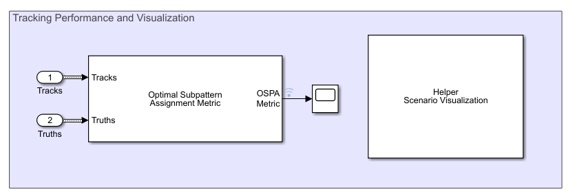
You assess the performance of each algorithm using the Optimal Subpattern Assignment (OSPA) metric. The OSPA metric aims to evaluate the performance of a tracking system with a scalar cost by combining different error components.
![]()
where ![]() ,
, ![]() , and
, and ![]() are localization, cardinality and labeling error components and p is the order of the OSPA metric. See
are localization, cardinality and labeling error components and p is the order of the OSPA metric. See trackOSPAMetric (Sensor Fusion and Tracking Toolbox) for more information.


You set the Distance type parameter to custom and define the distance function between a track and its associated ground truth as the helperExtendedTargetDistance helper function. This distance helper function captures position, velocity, dimension and yaw error between a track and an associated truth. The OSPA metric is shown in the scope block. Each unit on the x-axis represents 10 time steps in the scenario. Notice that the OSPA metric decreases and thus shows performance improvement when you switch from point object tracker to GGIW-PHD tracker and from GGIW-PHD tracker to GM-PHD tracker. The scenario is visualized using the Helper Scenario Visualization block, implemented using the MATLAB System (Simulink) block. Code for this block is defined in the helper class helperExtendedTargetTrackingDisplayBlk.
bdclose('ExtendedObjectTrackingInSimulink');
Summary
In this example you learned how to track objects that return multiple detections in a single sensor scan using different tracking approaches in Simulink environment. You also learned how to evaluate the performance of a tracking algorithm using the OSPA metric.
See Also
Scenario Reader | Driving Radar Data Generator | Vision Detection Generator | Multi-Object Tracker | Probability Hypothesis Density (PHD) Tracker (Sensor Fusion and Tracking Toolbox) | Optimal Subpattern Assignment Metric (Sensor Fusion and Tracking Toolbox)