Main Content

wmspca

Multiscale principal component analysis

    Description

    [xsim,qual,npc_out,decsim,pca_params] = wmspca(x,level,wname,npc_in) returns a simplified version xsim of the input matrix x obtained from the wavelet-based multiscale principal component analysis (PCA). The wavelet decomposition is performed using the decomposition level level and the wavelet wname.

    example

    [___] = wmspca(x,level,wname,'mode',extmode,npc_in) uses the specified discrete wavelet transform (DWT) extension mode extmode.

    [___] = wmspca(dec,npc_in) uses the wavelet decomposition structure dec. dec is expected to be the output of mdwtdec.

    Examples

    collapse all

    Use wavelet multiscale principal component analysis to denoise a multivariate signal.

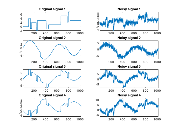
    Load the dataset consisting of four signals of length 1024. Plot the original signals and the signals with additive noise.

    load ex4mwden
    for i = 0:3
        subplot(4,2,2*i+1)
        plot(x_orig(:,i+1))
        axis tight
        title(['Original signal ',num2str(i+1)])
        subplot(4,2,2*i+2)
        plot(x(:,i+1))
        axis tight
        title(['Noisy signal ',num2str(i+1)])
    end

    Figure contains 8 axes objects. Axes object 1 with title Original signal 1 contains an object of type line. Axes object 2 with title Noisy signal 1 contains an object of type line. Axes object 3 with title Original signal 2 contains an object of type line. Axes object 4 with title Noisy signal 2 contains an object of type line. Axes object 5 with title Original signal 3 contains an object of type line. Axes object 6 with title Noisy signal 3 contains an object of type line. Axes object 7 with title Original signal 4 contains an object of type line. Axes object 8 with title Noisy signal 4 contains an object of type line.

    Perform the first multiscale wavelet PCA using the Daubechies least-asymmetric wavelet with four vanishing moments, sym4. Obtain the multiresolution decomposition down to level 5. Use the heuristic rule to decide how many principal components to retain.

    level = 5;
    wname = 'sym4';
    npc = 'heur';
    [x_sim,qual,npcA] = wmspca(x,level,wname,npc);

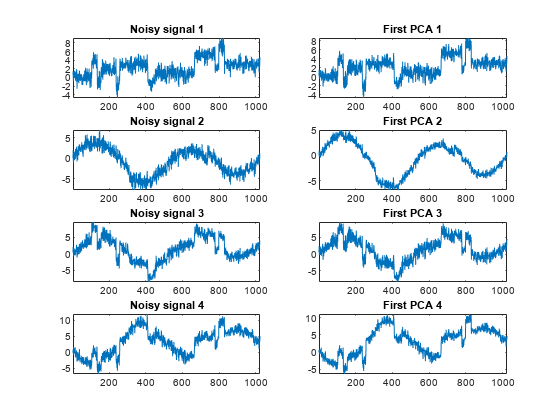
    Plot the result and examine the quality of the approximation.

    for i = 0:3
        subplot(4,2,2*i+1)
        plot(x(:,i+1))
        axis tight
        title(['Noisy signal ',num2str(i+1)])
        subplot(4,2,2*i+2)
        plot(x_sim(:,i+1))
        axis tight
        title(['First PCA ',num2str(i+1)])
    end

    Figure contains 8 axes objects. Axes object 1 with title Noisy signal 1 contains an object of type line. Axes object 2 with title First PCA 1 contains an object of type line. Axes object 3 with title Noisy signal 2 contains an object of type line. Axes object 4 with title First PCA 2 contains an object of type line. Axes object 5 with title Noisy signal 3 contains an object of type line. Axes object 6 with title First PCA 3 contains an object of type line. Axes object 7 with title Noisy signal 4 contains an object of type line. Axes object 8 with title First PCA 4 contains an object of type line.

    qual
    qual = 1×4
    
       97.4372   94.5520   97.7362   99.5219


    The quality results are all close to 100%. The npc vector gives the number of principal components retained at each level.

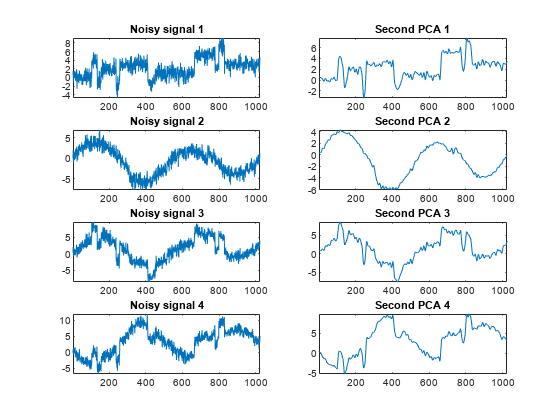
    Suppress the noise by removing the principal components at levels 1-3. Perform the multiscale PCA again.

    npcA(1:3) = zeros(1,3);
    [x_sim,qual,npcB] = wmspca(x,level,wname,npcA);

    Plot the result.

    for i = 0:3
        subplot(4,2,2*i+1)
        plot(x(:,i+1))
        axis tight
        title(['Noisy signal ',num2str(i+1)])
        subplot(4,2,2*i+2)
        plot(x_sim(:,i+1))
        axis tight
        title(['Second PCA ',num2str(i+1)])
    end

    Figure contains 8 axes objects. Axes object 1 with title Noisy signal 1 contains an object of type line. Axes object 2 with title Second PCA 1 contains an object of type line. Axes object 3 with title Noisy signal 2 contains an object of type line. Axes object 4 with title Second PCA 2 contains an object of type line. Axes object 5 with title Noisy signal 3 contains an object of type line. Axes object 6 with title Second PCA 3 contains an object of type line. Axes object 7 with title Noisy signal 4 contains an object of type line. Axes object 8 with title Second PCA 4 contains an object of type line.

    Input Arguments

    collapse all

    Multisignal, specified as a real-valued matrix. The matrix x contains P signals of length N stored column-wise (N > P).

    Data Types: double

    Level of decomposition, specified as a positive integer. wmspca does not enforce a maximum level restriction. Use wmaxlev to ensure that the wavelet coefficients are free from boundary effects. If boundary effects are not a concern, a good rule is to set level less than or equal to fix(log2(length(N))), where N is the signal length.

    Data Types: double

    Wavelet, specified as a character vector or string scalar. The wavelet must be orthogonal or biorthogonal. Orthogonal and biorthogonal wavelets are designated as type 1 and type 2 wavelets respectively in the wavelet manager, wavemngr.

    • Valid built-in orthogonal wavelet families are: Best-localized Daubechies ("bl"), Beylkin ("beyl"), Coiflets ("coif"), Daubechies ("db"), Fejér-Korovkin ("fk"), Haar ("haar"), Han linear-phase moments ("han"), Morris minimum-bandwidth ("mb"), Symlets ("sym"), and Vaidyanathan ("vaid").

    • Valid built-in biorthogonal wavelet families are: Biorthogonal Spline ("bior"), and Reverse Biorthogonal Spline ("rbio").

    For a list of wavelets in each family, see wfilters. You can also use waveinfo with the wavelet family short name. For example, waveinfo("db"). Use wavemngr("type",wn) to determine if the wavelet wn is orthogonal (returns 1) or biorthogonal (returns 2). For example, wavemngr("type","db6") returns 1.

    Principal components parameter, specified as a vector, character vector, or string scalar.

    • If npc_in is a vector, then it must be of length level+2. The vector npc_in contains the number of retained principal components for each PCA performed:

      • npc_in(d) is the number of retained noncentered principal components for details at level d, for 1 ≤ dlevel.

      • npc_in(level+1) is the number of retained non-centered principal components for approximations at level level.

      • npc_in(level+2) is the number of retained principal components for final PCA after wavelet reconstruction.

      npc_in must be such that 0 ≤ npc_in(d)P, where P is the number of signals, for 1 ≤ dlevel+2.

    • If npc_in is "kais", then the number of retained principal components is selected automatically using Kaiser's rule. Kaiser's rule keeps the components associated with eigenvalues exceeding the mean of all eigenvalues.

    • If npc_in is "heur", then the number of retained principal components is selected automatically using the heuristic rule. The heuristic rule keeps the components associated with eigenvalues greater than 0.05 times the sum of all eigenvalues.

    • If npc_in is "nodet", then the details are "killed" and all the approximations are retained.

    Data Types: double | string | char

    Extension mode used when performing the wavelet decomposition, specified as:

    mode

    DWT Extension Mode

    'zpd'

    Zero extension

    'sp0'

    Smooth extension of order 0

    'spd' (or 'sp1')

    Smooth extension of order 1

    'sym' or 'symh'

    Symmetric extension (half point): boundary value symmetric replication

    'symw'

    Symmetric extension (whole point): boundary value symmetric replication

    'asym' or 'asymh'

    Antisymmetric extension (half point): boundary value antisymmetric replication

    'asymw'

    Antisymmetric extension (whole point): boundary value antisymmetric replication

    'ppd', 'per'

    Periodized extension

    If the signal length is odd and mode is 'per', an extra sample equal to the last value is added to the right and the extension is performed in 'ppd' mode. If the signal length is even, 'per' is equivalent to 'ppd'. This rule also applies to images.

    The global variable managed by dwtmode specifies the default extension mode. Use dwtmode to determine the extension modes.

    Wavelet decomposition structure of a multisignal, specified as a structure. dec is expected to be the output of mdwtdec. The multisignal input of mdwtdec is a matrix A, where the signals are arranged column-wise. If A is N-by-P, then N must be greater than P.

    Data Types: double

    Output Arguments

    collapse all

    Simplified multivariate multisignal, returned as a matrix. The dimensions of xsim equal the dimensions of x.

    Data Types: double

    Quality of column reconstructions, returned as a vector of length P, where P is equal to size(x,2). qual contains the quality of column reconstructions given by the relative mean square errors in percent.

    Data Types: double

    Number of retained principal components, returned as a vector. If npc_in is a vector, then npc_out equals npc_in.

    Data Types: double

    Wavelet decomposition of the simplified multisignal xsim, returned as a structure with the following fields:

    • dirDec'c' (column), indicator of decomposition direction

    • level — Level of wavelet decomposition

    • wname — Wavelet name

    • dwtFilters — Structure with four fields:

      • LoD — Lowpass decomposition filter

      • HiD — Highpass decomposition filter

      • LoR — Lowpass reconstruction filter

      • HiR — Highpass reconstruction filter

    • dwtEXTM — DWT extension mode

    • dwtShift — DWT shift parameter (0 or 1)

    • dataSize — Size of x

    • ca — Approximation coefficients at level level

    • cd — Cell array of detail coefficients, from level 1 to level level

    ca and cd{k}, for k from 1 to level, are matrices, where the coefficients are stored as columns.

    PCA parameters, returned as a structure array of length level+2, where:

    • pca_params(d).pc is a P-by-P matrix of principal components. The columns are stored in descending order of the variances.

    • pca_params(d).variances is the principal component variances vector.

    • pca_params(d).npc = npc_out

    Algorithms

    The multiscale principal components generalizes the usual PCA of a multivariate signal seen as a matrix by performing simultaneously a PCA on the matrices of details of different levels. In addition, a PCA is performed also on the coarser approximation coefficients matrix in the wavelet domain as well as on the final reconstructed matrix. By selecting conveniently the numbers of retained principal components, interesting simplified signals can be reconstructed.

    References

    [1] Bakshi, Bhavik R. “Multiscale PCA with Application to Multivariate Statistical Process Monitoring.” AIChE Journal 44, no. 7 (July 1998): 1596–1610. https://doi.org/10.1002/aic.690440712.

    Version History

    Introduced in R2006b