2-D FFT
Compute 2-D fast Fourier transform (FFT)

Libraries:
Computer Vision Toolbox /
Transforms
Description
The 2-D FFT block computes the discrete Fourier transform (DFT) of a two-dimensional input matrix using the fast Fourier transform (FFT) algorithm. The equation for the two-dimensional DFT F(m, n) of an M-by-N input matrix, f(x, y), is:
where and .
The block supports FFT implementation based on the FFTW library and an implementation based on a collection of Radix-2 algorithms. You can either manually select one of these implementations or let the block select one automatically.
Examples
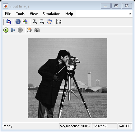
Filter Image in Frequency Domain
Apply Gaussian lowpass filter to an image using the 2-D FFT block.
Ports
Input
Output
Parameters
Block Characteristics
Data Types |
|
Multidimensional Signals |
|
Variable-Size Signals |
|
More About
Two numbers are bit-reversed values of each other when the binary representation of one
is the mirror image of the binary representation of the other. For example, in a three-bit
system, one and four are bit-reversed values of each other because the three-bit binary
representation of one, 001, is the mirror image of the three-bit binary
representation of four, 100. The diagram shows the row indices in linear
order. To put them in bit-reversed order:
Translate the indices into their binary representations with the minimum number of bits. In this example, the minimum number of bits is three because the binary representation of the largest row index, 7, is
111.Find the mirror image of each binary entry, and write it beside the original binary representation.
Translate each binary mirror image to its decimal representation.
The row indices now appear in bit-reversed order.

When you select the Output in bit-reversed order parameter of the 2-D FFT block, the block bit-reverses the order of both the rows and columns. All output values remain the same, but they appear in a different order.
These diagrams show the data types used in the 2-D FFT block for fixed-point signals. The block first casts inputs to the output data type and stores them in the output buffer. Each butterfly stage then processes signals in the accumulator data type, with the final butterfly casting its output back into the output data type. The block multiplies by a twiddle factor before each butterfly stage, in a decimation-in-time FFT, and after each butterfly stage in a decimation-in-frequency FFT.
The multiplier output appears in the accumulator data type because both of the inputs to the multiplier are complex. For details on the complex multiplication performed, refer to Multiplication Data Types.
Algorithms
References
[1] “FFTW Home Page.” Accessed February 23, 2022. https://www.fftw.org/.
[2] Frigo, M., and S.G. Johnson. “FFTW: An Adaptive Software Architecture for the FFT.” In Proceedings of the 1998 IEEE International Conference on Acoustics, Speech and Signal Processing, ICASSP ’98 (Cat. No.98CH36181), 3:1381–84. Seattle, WA, USA: IEEE, 1998. https://doi.org/10.1109/ICASSP.1998.681704.
Extended Capabilities
Version History
Introduced before R2006a