Model Reference Adaptive Control of Satellite Spin
This example shows how to control satellite spin using model reference adaptive control (MRAC) to make the unknown controlled system match an ideal reference model. The satellite system is modeled in Simulink® and the MRAC controller is implemented using the Model Reference Adaptive Control block provided by Simulink Control Design™ software.
Satellite-Spin Control System
In the model for this example, the cylindrical body of the satellite spins around its axis of symmetry (z axis) with constant angular rate [1]. The goal is to independently control the angular rates and around the and axes using torques and . The equations of motion produce a second-order model with two inputs and two outputs.
In this system, the controller does not observe the plant states directly. Instead, it views the states indirectly through following measurement model.
For this example, assume that the actual plant model is unknown and that the MRAC controller uses the following nominal model of the plant dynamics.
Given this uncertain nonlinear system, your goal is to design a controller that enables the system to track the following decoupled reference model.
Here:
is the reference model state vector.
contains the angular rate reference signals.
Define Nominal and Reference Models
Define the dynamic model for the satellite system. For this system, A represents the true state matrix.
a = 10;                % System Constant
A = [0 a;-a -a/2];     % True model parameters
B = eye(2);
C = [1 a;-a 1];
D = zeros(2,2);
Specify a plant mismatch matrix. This matrix is subtracted from the true A matrix to define the nominal plant used by the controller. The goal of the controller is to model this plant uncertainty.
deltaA = [0 0.5*a; -0.5*a 0]; % Plant mismatchThe reference system is the following stable second order system.
Am = [-5 0; 0 -5];    % Second-order decoupled integrator model
Bm = diag([5 5]);     % Nominal control effective matrix
Define the initial conditions for the satellite spin rates and reference model states.
x1_0 = 0.5;     % Initial x-axis angular rate (rad/s)
x2_0 = 0.5;     % Initial y-axis angular rate (rad/s)
xm_0 = [0;0];   % Initial conditions of the reference plant model
Model Reference Adaptive Control Structure
The goal of the MRAC controller is to achieve asymptotic convergence of the tracking error .
The MRAC controller has the following structure.
Here:
contains feedback control gains.
contains feedforward control gains.
is an adaptive control term that cancels the model uncertainty.
The Model Reference Adaptive Control block adjusts the adaptive control term to achieve the desired reference model tracking. Optionally, you can also adapt the feedback and feedforward control gains.
For this example, the controller adapts the feedback gains and keeps the feedforward gains static.
The initial feedback gain and the static feedforward gain are computed to satisfy the following model matching condition:
Specify the computed controller gains and the feedback gain learning rate.
Kx = -place(A,B,eig(Am));  % State feedback gain for pole placement
gain_kx = 1;               % Feedback gain learning rate
Kr = Bm;                   % Feedforward gain for ref model matching
Configure Uncertainty Estimation Parameters
The MRAC controller estimates the model uncertainty online and generates an adaptive control action that cancels the uncertainty to recover the nominal system for the baseline controller. The adaptive control term models the system uncertainty using the following model.
Here:
contains the network weights that are adjusted by the controller.
is the uncertainty model feature vector.
Using the Model Reference Adaptive Control block, you can select one of the following feature vector definitions.
System states, where
Radial basis functions with Gaussian kernels
Custom features provided by an optional input port.
For this example, the controller is configured to use the system states as the disturbance model features.
Define the model estimation learning rate gamma_w and tracking error weight Q.
gamma_w = 100;  % Learning rate
Q = 10;         % Tracking error weight
Simulate Controller
Open the Simulink model of the satellite-spin control system.
mdl = "satellitespin";
open_system(mdl)
Simulate the model.
Tf = 35;        % Duration (s)
sim(mdl);


View the controller performance by comparing the spin response and spin-rate response to their respective reference signals.
open_system(mdl + "/Scope1")
open_system(mdl + "/Scope3")
The MRAC controller tracks the reference signals well. The first step response has an initial transient, which reduces in size as the disturbance estimate of the controller improves.
View the uncertainty estimated by the controller and compare it to the true uncertainty.
open_system(mdl + "/Scope2")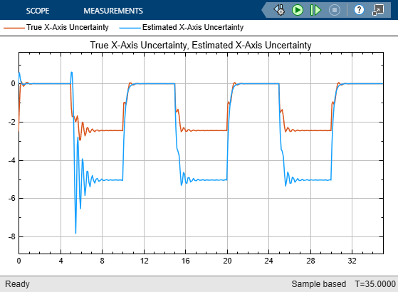
open_system(mdl + "/Scope4")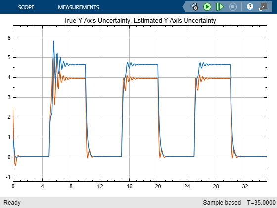
The controller estimates an accurate y-axis uncertainty model. The uncertainty model for the x-axis has the correct sign, though the magnitude is lower than that of the true uncertainty. Both uncertainty models show significant transients in the uncertainty estimate, especially during the first step change in the reference signals.
To reduce the transients in the estimated uncertainty responses, you can reduce the value of the tracking error rate Q. For example, reduce the value of Q to 1 and simulate the model.
Q = 1;
sim(mdl);
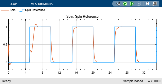
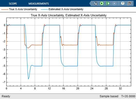
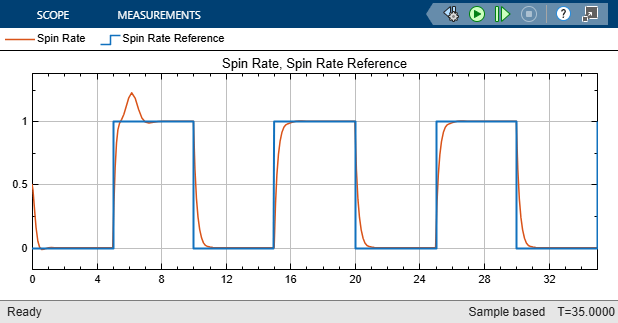
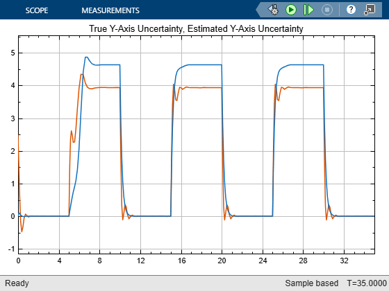
The model estimate responses have fewer transients. The tradeoff is that the spin and spin-rate responses have longer settling times.
Reference
[1] Zhou, Kemin, John Comstock Doyle, and K. Glover. Robust and Optimal Control. Englewood Cliffs, N.J: Prentice Hall, 1996.