Estimate Battery Model Parameters from HPPC Data
This example shows how to estimate the model parameters for a battery equivalent circuit model (ECM) from hybrid pulse power characterization (HPPC) data using Simscape™ Battery™. HPPC is a valuable technique in the battery industry and is one of the most common battery tests performed both at single-cell level or at system level. This technique involves applying a series of constant current pulses to a battery and measuring its terminal voltage and temperature responses at different operating conditions. There are multiple key operating conditions, including the initial battery soak temperature, initial state of charge (SOC), current or load, current directionality such as charge or discharge, state of health (SOH) or remaining capacity, and load frequency. The measured voltage response from each current pulse contains valuable information regarding the internal resistance or impedance of the battery.
In this example, you first define an hppcTest object that allows you to visualize, tabulate, and manipulate the different constant current pulses inside your HPPC data. The HPPCTest object contains a summary of all the current pulses performed in a single HPPC test program. This object automatically identifies each constant current pulse and tabulates it for inspection and preparation for the parameter estimation process as an optional data pre-processing step. This HPPC test data must be in a MAT file format and must contain time, current, and voltage signals. Optionally, you can specify the temperature, charge, and SOC.
You then estimate the parameters for a battery ECM that best match the terminal voltage response of the battery. The key outputs from the parameter estimation process are 1-D, 2-D, or 3-D parameter look-up tables. You can use these tables for control, as part of battery management system (BMS) algorithms, or for simulation, as parameters for the Battery Equivalent Circuit block.
Finally, this example shows you how to automatically parameterize the Battery Equivalent Circuit block to run battery simulations.

Create and Visualize HPPCTest Objects
An HPPCTest object automatically identifies all individual constant current pulses inside an HPPC test file. To create an HPPCTest object, first load the HPPC data into the MATLAB® workspace.
load("testDataBAKcells/hppcDataBAKcell25degC.mat","hppcData")
To create an HPPCTest object, use the hppcTest function. By default, the HPPCTest object assumes that the time, voltage, and current columns are named "Time", "Voltage", and "Current", respectively. If these variables have different column name identifiers, you can specify them by using the optional name-value arguments.
hppcExp25degC = hppcTest(hppcData,...
    TimeVariable="time (s)", ...
    VoltageVariable="voltage (V)", ...
    CurrentVariable="current (A)", ...
    Capacity=2.84, ...
    InitialSOC=0.055);
The HPPCTest object automatically calculates the battery SOC at every time step across the experiment, according to the input current measurement. The object uses these calculated SOC values to define the SOC breakpoints for every constant current pulse. The TestSummary property contains a summary of these SOC breakpoints as well as all other temperature and current breakpoints identified from the data. Optionally, to improve the accuracy of the calculation of the SOC, the hppcTest function allows you to specify the battery capacity, the test initial SOC, and these column vectors:
Charge— If you specify this column variable and theStateOfChargevariable is empty, theHPPCTestobject uses the values in this column to calculate the SOC breakpoints.StateOfCharge— if you specify this column variable, theHPPCTestobject uses the values in this column to calculate the SOC breakpoints.
To visualize a summary of the test and the identified charge and discharge pulses, use the plot function.
plot(hppcExp25degC)

The function automatically identifies the charge and discharge constant current pulses from the data according to these properties:
ValidPulseDurationRange— Valid pulse duration range that indicates whether a pulse is valid and must be stored in theTestSummaryproperty table. Decreasing the upper bound to values lower than 60 seconds ensures that very long discharges, such as capacity checks, are not included in the final list of pulses for estimation. Increasing the lower bound for this property to values greater than one or two seconds, ensures that the function excludes potential noise, outlier currents, or abnormally short pulses from the final list of pulses for estimation.ValidVoltageRange— Valid battery voltage range that indicates whether a pulse is valid and must be stored in theTestSummaryproperty table.CurrentOnThreshold— Threshold current value that indicates whether a charge or a discharge is occurring. This value is important for experiments where the rest or baseline current is not equal to zero.NumSamplesRequirement— Number of sequential points, specified as a scalar, at which the current must be greater than theCurrentOnThresholdvalue to signify the presence of a charge or discharge pulse.
You can customize these properties with your individual options to filter out or only select the pulses that you want to use for parameter estimation. Optionally, you can also remove pulses manually from the TestSummary table after object creation by using the removePulse function.
To view a summary of all the identified pulses, use the TestSummary property.
disp(hppcExp25degC.TestSummary)
    PulseID    Directionality      SOC           HPPCData         PulseDuration    PseudoOCV_V    MaximumVoltage    MinimumVoltage    Current_A    C_rate    PulseStartIndex    PulseEndIndex    Temperature_degC
    _______    ______________    ________    _________________    _____________    ___________    ______________    ______________    _________    ______    _______________    _____________    ________________

       1        "Discharge"        0.9866    {701×6 timetable}         30            4.1745           4.1745            3.7846         -6.1869     2.1785           354              1055               25
       2        "Discharge"       0.87612    {701×6 timetable}         30            4.0837           4.0837            3.7479          -6.187     2.1785          2702              3403               25
       3        "Discharge"       0.76566    {702×6 timetable}         30            4.0132           4.0132            3.6652         -6.1867     2.1784          5049              5751               25
       4        "Discharge"       0.65521    {701×6 timetable}         30            3.9226           3.9226            3.5775         -6.1868     2.1784          7398              8099               25
       5        "Discharge"       0.54476    {701×6 timetable}         30             3.846            3.846            3.4942         -6.1868     2.1784          9746             10447               25
       6        "Discharge"       0.43431    {701×6 timetable}         30            3.7353           3.7353            3.4001         -6.1871     2.1785         12094             12795               25
       7        "Discharge"       0.32386    {701×6 timetable}         30              3.65             3.65            3.3236         -6.1867     2.1784         14442             15143               25
       8        "Discharge"        0.2134    {701×6 timetable}         30            3.6015           3.6015            3.2652         -6.1869     2.1785         16790             17491               25
       9        "Discharge"       0.10295    {701×6 timetable}         30            3.5507           3.5507            3.1931         -6.1869     2.1785         19138             19839               25
      10        "Charge"           0.9684    {502×6 timetable}         10            4.1158           4.3889            4.1158          4.6393     1.6336          1055              1557               25
      11        "Charge"          0.85795    {502×6 timetable}         10             4.057           4.3001             4.057          4.6406      1.634          3403              3905               25
      12        "Charge"          0.74749    {502×6 timetable}         10            3.9674           4.2113            3.9674          4.6394     1.6336          5751              6253               25
      13        "Charge"          0.63704    {502×6 timetable}         10            3.8751           4.1175            3.8751          4.6396     1.6337          8099              8601               25
      14        "Charge"          0.52659    {502×6 timetable}         10            3.7905           4.0355            3.7905          4.6396     1.6337         10447             10949               25
      15        "Charge"          0.41614    {502×6 timetable}         10            3.6936           3.9339            3.6936          4.6405      1.634         12795             13297               25
      16        "Charge"          0.30569    {502×6 timetable}         10            3.6224           3.8602            3.6224          4.6396     1.6337         15143             15645               25
      17        "Charge"          0.19523    {502×6 timetable}         10            3.5695           3.8109            3.5695          4.6397     1.6337         17491             17993               25
      18        "Charge"         0.084783    {502×6 timetable}         10            3.5098           3.7597            3.5098          4.6397     1.6337         19839             20341               25
You can visualize the voltage response for specific pulses from the TestSummary table by using the plotPulse function. The plotPulse function optionally accepts a second argument that specifies the index for the pulses to be visualized and inspected for abnormalities. This index refers to the PulseID column in the TestSummary property table. You can specify this index as a scalar or vector.
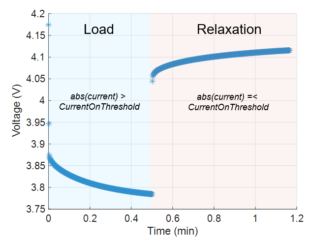
A constant current pulse involves two key phases: the load segment and the relaxation segment. You can use these segments to characterize the performance, capacity, and internal resistance of your battery. Typically, the battery ECM parameters are different depending on which segment you use for the parameter estimation process.
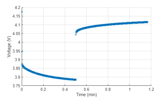
Plot the first pulse in the HPPCTest object using the plotPulse function. Until 0.5 minutes, the battery is under load and the absolute current exceeds the value of the CurrentOnThreshold property. After 0.5 minutes, the pulse enters the relaxation segment where the absolute current is less than or equal to the value of the CurrentOnThreshold property.
plotPulse(hppcExp25degC)
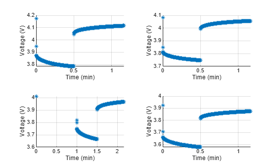
You can visualize the different pulses in a grid layout by defining a vector as the second argument of the plotPulse function.
plotPulse(hppcExp25degC,1:4)
You can also remove individual pulses that behave abnormally or do not meet your requirements, including nonlinear voltage response, missing points, voltage outliers, or abnormal dispersion. In this HPPC dataset, the third pulse might be missing the initial rest voltage at the beginning of the pulse. Remove it from the parameter estimation process by using the removePulse function.
removePulse(hppcExp25degC,3)
Inspect the updated TestSummary property. Notice that there are now only 17 pulses in the table.
disp(hppcExp25degC.TestSummary)
    PulseID    Directionality      SOC           HPPCData         PulseDuration    PseudoOCV_V    MaximumVoltage    MinimumVoltage    Current_A    C_rate    PulseStartIndex    PulseEndIndex    Temperature_degC
    _______    ______________    ________    _________________    _____________    ___________    ______________    ______________    _________    ______    _______________    _____________    ________________

       1        "Discharge"        0.9866    {701×6 timetable}         30            4.1745           4.1745            3.7846         -6.1869     2.1785           354              1055               25
       2        "Discharge"       0.87612    {701×6 timetable}         30            4.0837           4.0837            3.7479          -6.187     2.1785          2702              3403               25
       3        "Discharge"       0.65521    {701×6 timetable}         30            3.9226           3.9226            3.5775         -6.1868     2.1784          7398              8099               25
       4        "Discharge"       0.54476    {701×6 timetable}         30             3.846            3.846            3.4942         -6.1868     2.1784          9746             10447               25
       5        "Discharge"       0.43431    {701×6 timetable}         30            3.7353           3.7353            3.4001         -6.1871     2.1785         12094             12795               25
       6        "Discharge"       0.32386    {701×6 timetable}         30              3.65             3.65            3.3236         -6.1867     2.1784         14442             15143               25
       7        "Discharge"        0.2134    {701×6 timetable}         30            3.6015           3.6015            3.2652         -6.1869     2.1785         16790             17491               25
       8        "Discharge"       0.10295    {701×6 timetable}         30            3.5507           3.5507            3.1931         -6.1869     2.1785         19138             19839               25
       9        "Charge"           0.9684    {502×6 timetable}         10            4.1158           4.3889            4.1158          4.6393     1.6336          1055              1557               25
      10        "Charge"          0.85795    {502×6 timetable}         10             4.057           4.3001             4.057          4.6406      1.634          3403              3905               25
      11        "Charge"          0.74749    {502×6 timetable}         10            3.9674           4.2113            3.9674          4.6394     1.6336          5751              6253               25
      12        "Charge"          0.63704    {502×6 timetable}         10            3.8751           4.1175            3.8751          4.6396     1.6337          8099              8601               25
      13        "Charge"          0.52659    {502×6 timetable}         10            3.7905           4.0355            3.7905          4.6396     1.6337         10447             10949               25
      14        "Charge"          0.41614    {502×6 timetable}         10            3.6936           3.9339            3.6936          4.6405      1.634         12795             13297               25
      15        "Charge"          0.30569    {502×6 timetable}         10            3.6224           3.8602            3.6224          4.6396     1.6337         15143             15645               25
      16        "Charge"          0.19523    {502×6 timetable}         10            3.5695           3.8109            3.5695          4.6397     1.6337         17491             17993               25
      17        "Charge"         0.084783    {502×6 timetable}         10            3.5098           3.7597            3.5098          4.6397     1.6337         19839             20341               25
Modify SOC Breakpoints
If you do not have information about the battery capacity, SOC, or charge, you can optionally modify the SOC breakpoint values inside the TestSummary property table by using the setChargeSOCs and setDischargeSOCs functions.
 setChargeSOCs(hppcExp25degC,[1,0.9,0.8,0.6,0.5,0.4,0.3,0.2,0.1]);
 setDischargeSOCs(hppcExp25degC,[1,0.9,0.7,0.5,0.4,0.3,0.2,0.1]);
Inspect the updated TestSummary property table. Notice that the functions modified the SOC breakpoints.
disp(hppcExp25degC.TestSummary)
    PulseID    Directionality    SOC        HPPCData         PulseDuration    PseudoOCV_V    MaximumVoltage    MinimumVoltage    Current_A    C_rate    PulseStartIndex    PulseEndIndex    Temperature_degC
    _______    ______________    ___    _________________    _____________    ___________    ______________    ______________    _________    ______    _______________    _____________    ________________

       1        "Discharge"        1    {701×6 timetable}         30            4.1745           4.1745            3.7846         -6.1869     2.1785           354              1055               25
       2        "Discharge"      0.9    {701×6 timetable}         30            4.0837           4.0837            3.7479          -6.187     2.1785          2702              3403               25
       3        "Discharge"      0.7    {701×6 timetable}         30            3.9226           3.9226            3.5775         -6.1868     2.1784          7398              8099               25
       4        "Discharge"      0.5    {701×6 timetable}         30             3.846            3.846            3.4942         -6.1868     2.1784          9746             10447               25
       5        "Discharge"      0.4    {701×6 timetable}         30            3.7353           3.7353            3.4001         -6.1871     2.1785         12094             12795               25
       6        "Discharge"      0.3    {701×6 timetable}         30              3.65             3.65            3.3236         -6.1867     2.1784         14442             15143               25
       7        "Discharge"      0.2    {701×6 timetable}         30            3.6015           3.6015            3.2652         -6.1869     2.1785         16790             17491               25
       8        "Discharge"      0.1    {701×6 timetable}         30            3.5507           3.5507            3.1931         -6.1869     2.1785         19138             19839               25
       9        "Charge"           1    {502×6 timetable}         10            4.1158           4.3889            4.1158          4.6393     1.6336          1055              1557               25
      10        "Charge"         0.9    {502×6 timetable}         10             4.057           4.3001             4.057          4.6406      1.634          3403              3905               25
      11        "Charge"         0.8    {502×6 timetable}         10            3.9674           4.2113            3.9674          4.6394     1.6336          5751              6253               25
      12        "Charge"         0.6    {502×6 timetable}         10            3.8751           4.1175            3.8751          4.6396     1.6337          8099              8601               25
      13        "Charge"         0.5    {502×6 timetable}         10            3.7905           4.0355            3.7905          4.6396     1.6337         10447             10949               25
      14        "Charge"         0.4    {502×6 timetable}         10            3.6936           3.9339            3.6936          4.6405      1.634         12795             13297               25
      15        "Charge"         0.3    {502×6 timetable}         10            3.6224           3.8602            3.6224          4.6396     1.6337         15143             15645               25
      16        "Charge"         0.2    {502×6 timetable}         10            3.5695           3.8109            3.5695          4.6397     1.6337         17491             17993               25
      17        "Charge"         0.1    {502×6 timetable}         10            3.5098           3.7597            3.5098          4.6397     1.6337         19839             20341               25
Estimate Battery Model Parameters
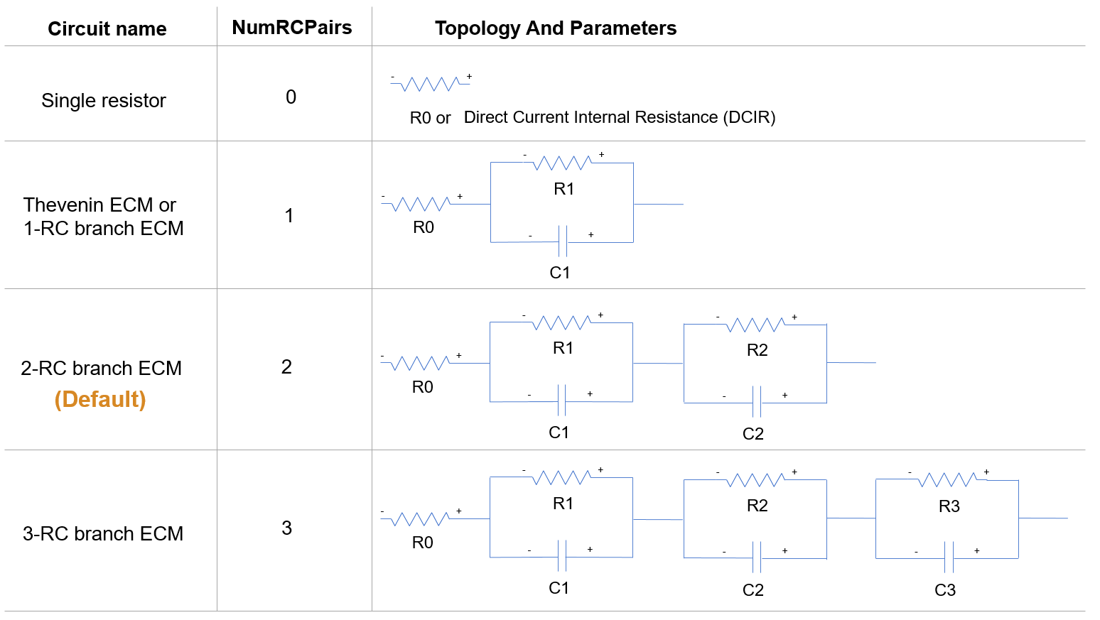
The process of parameter estimation involves minimizing the error between the predicted voltage output of the ECM and the measured battery voltage response from the HPPC test. This table shows the most typical ECMs used to represent the impedance of a battery:
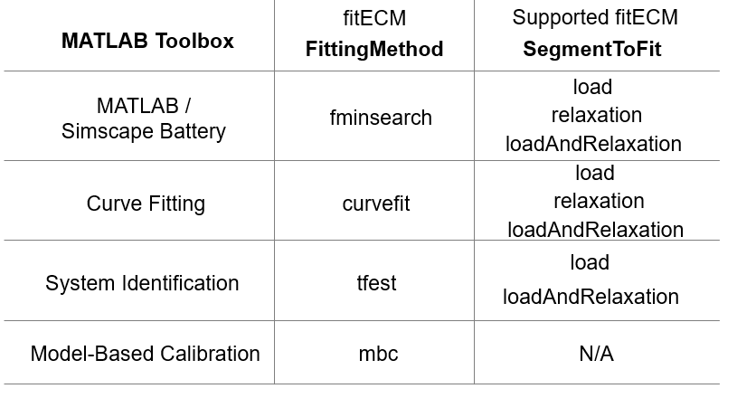
To minimize the error, you iteratively adjust the model parameters, such as R0, R1, and C1, until you achieve a satisfactory error between the measured voltage and a simulated voltage. There are several techniques in MATLAB that provide this functionality inside the Model-Based Calibration Toolbox™, System Identification Toolbox™, and Curve Fitting Toolbox™. In this example, you estimate the parameters of the battery model by using an optimization-based fitting method implemented in Simscape Battery. This fitting method utilizes a custom implementation of the fminsearch function.
The battery ECM parameters for a specific operating point can be different depending on which segment or section of the current pulse you use for the parameter estimation process. The load-segment parameters suit most applications. However, the best estimation segment depends on the specific end application of the battery ECM. Some methods are better suited to estimate parameters for a given segment, for example the System Identification Toolbox tfest function works best for fitting load-only dynamics. This table contains a summary of the supported options for the FittingMethod and SegmentToFit arguments of the fitecm function, depending on the chosen toolbox or method.
Estimate Parameters for Single Current Pulse
There are a total of 17 constant current pulses inside the hppcExp25degC object. To estimate the ECM parameters for a specific constant current pulse profile in your test data, first define the index of the pulse you want to find the ECM parameters for. This index relates to a specific row in the TestSummary property table.
pulseIndex = 5;
To find the ECM parameters, use the fitECM function. This function requires the HPPC test data as input. The default value for the FittingMethod argument is "fminsearch", which is the optimization method implemented in Simscape Battery. The default value for the SegmentToFit argument focuses on the relaxation section of the constant current pulse. Different options for the FittingMethod argument of the fitECM function allow you to perform the parameter estimation process for different segments of the pulse.
batteryEcm = fitECM(hppcExp25degC.TestSummary.HPPCData{pulseIndex}(:,1:2), SegmentToFit="loadAndRelaxation"); The fitECM function returns an ecm object. View the ECM topology and other properties of the ECM object.
disp(batteryEcm)
  ECM with properties:

                          NumRCPairs: 2
                       NumParameters: 5
                       ParameterList: ["R0"    "R1"    "C1"    "R2"    "C2"]
                    CircuitImpedance: "R0 + 1/(i*w*C1+1/R1) + 1/(i*w*C2+1/R2)"
                     ParameterValues: [0.0408 0.0020 555.9667 0.0129 1.6035e+03]
                ModelParameterTables: [1×1 struct]
            ResistanceSOCBreakpoints: [0 0.1000 0.2000 0.3000 0.4000 0.5000 0.6000 0.7000 0.8000 0.9000 1] (1)
    ResistanceTemperatureBreakpoints: [278 293 313] (K)
        ResistanceCurrentBreakpoints: 1 (A)

Show all properties
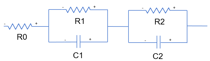
You can define optional name-value arguments for the fitECM function. For example, the ECM name-value argument specifies the desired ECM circuit topology you want to use to fit the data. If you do not specify this argument, the fitECM function uses this 2-RC branch ECM topology:
Use the plot function to visualize the measured and the simulated battery ECM voltage response. The plot function calculates the simulated battery ECM voltage response by assuming a constant open-circuit voltage value. In most cases, including a dynamic open-circuit voltage curve during the simulation improves the accuracy of the verification plot.
plot(batteryEcm)
Estimate Parameters for Sequence of Pulses
To estimate the ECM parameters for all the pulses inside a specific HPPCTest object, use the fitECM function and specify the entire HPPCTest object as input.
batteryEcm = fitECM(hppcExp25degC, SegmentToFit="loadAndRelaxation"); Display the parameters and estimation error by using the TestParameterTables property of the batteryEcm object.
disp(batteryEcm.TestParameterTables)
                TestBreakpoints: [1×1 struct]
       ChargeOpenCircuitVoltage: [3.5098 3.5695 3.6224 3.6936 3.7905 3.8751 3.9674 4.0570 4.1158]
                       ChargeR0: [0.0390 0.0382 0.0378 0.0392 0.0371 0.0369 0.0370 0.0397 0.0403]
                       ChargeR1: [0.0072 0.0067 0.0069 0.0049 0.0066 0.0065 0.0067 0.0052 0.0091]
                     ChargeTau1: [0.3751 0.3774 0.3982 0.3797 0.3286 0.3317 0.3874 0.3967 0.3551]
                       ChargeC1: [51.9419 56.5704 57.6792 76.7624 49.7476 51.0375 58.1648 76.3596 39.2237]
                       ChargeR2: [0.0103 0.0095 0.0644 0.0117 0.0129 0.0115 0.0114 0.0089 0.0154]
                     ChargeTau2: [9.5365 9.4661 24.1822 10.3457 8.3771 8.2633 8.6700 8.5273 9.3994]
                       ChargeC2: [921.5608 995.1325 375.6581 883.1525 649.5546 715.9945 761.9383 962.1568 612.1307]
                    ChargeFitPc: [2.3798e-05 2.1926e-05 8.9156e-05 2.5623e-05 2.9595e-05 2.7463e-05 2.9163e-05 2.8058e-05 3.7073e-05]
    DischargeOpenCircuitVoltage: [3.5507 3.6015 3.6500 3.7353 3.8460 3.9226 4.0837 4.1745]
                    DischargeR0: [0.0433 0.0418 0.0411 0.0408 0.0407 0.0406 0.0422 0.0407]
                    DischargeR1: [0.0017 0.0015 0.0016 0.0020 0.0024 0.0024 0.0023 0.0080]
                  DischargeTau1: [1.0136 1.0639 1.0778 1.1318 1.1306 1.1331 1.1418 0.6206]
                    DischargeC1: [587.1147 686.9393 670.4352 556.3512 467.1310 475.4616 489.4226 77.6454]
                    DischargeR2: [0.0180 0.0141 0.0122 0.0129 0.0146 0.0138 0.0108 0.0127]
                  DischargeTau2: [23.0014 21.2042 20.0352 20.7300 20.4551 19.9010 17.9218 15.9518]
                    DischargeC2: [1.2760e+03 1.5031e+03 1.6366e+03 1.6042e+03 1.3996e+03 1.4436e+03 1.6628e+03 1.2560e+03]
                 DischargeFitPc: [2.7466e-05 1.9487e-05 2.0726e-05 2.9118e-05 4.3007e-05 4.1371e-05 3.7379e-05 1.6776e-04]
The parameters inside the TestParameterTables property are different from the parameters inside the ModelParameterTables property. The ECM object determines the parameters inside the ModelParameterTables property by using the ECM object breakpoints you specify. The ECM object determines the parameters inside the TestParameterTables property by using the test conditions. View the model parameter tables by using the ModelParameterTables property.
disp(batteryEcm.ModelParameterTables)
       ChargeOpenCircuitVoltage: [3.5098 3.5098 3.5695 3.6224 3.6936 3.7905 3.8751 3.8751 3.9674 4.0570 4.1158]
                       ChargeR0: [0.0390 0.0390 0.0382 0.0378 0.0392 0.0371 0.0369 0.0369 0.0370 0.0397 0.0403]
                       ChargeR1: [0.0072 0.0072 0.0067 0.0069 0.0049 0.0066 0.0065 0.0065 0.0067 0.0052 0.0091]
                     ChargeTau1: [0.3751 0.3751 0.3774 0.3982 0.3797 0.3286 0.3317 0.3317 0.3874 0.3967 0.3551]
                       ChargeC1: [51.9419 51.9419 56.5704 57.6792 76.7624 49.7476 51.0375 51.0375 58.1648 76.3596 39.2237]
                       ChargeR2: [0.0103 0.0103 0.0095 0.0644 0.0117 0.0129 0.0115 0.0115 0.0114 0.0089 0.0154]
                     ChargeTau2: [9.5365 9.5365 9.4661 24.1822 10.3457 8.3771 8.2633 8.2633 8.6700 8.5273 9.3994]
                       ChargeC2: [921.5608 921.5608 995.1325 375.6581 883.1525 649.5546 715.9945 715.9945 761.9383 962.1568 612.1307]
                    ChargeFitPc: [2.3798e-05 2.3798e-05 2.1926e-05 8.9156e-05 2.5623e-05 2.9595e-05 2.7463e-05 2.7463e-05 2.9163e-05 2.8058e-05 3.7073e-05]
    DischargeOpenCircuitVoltage: [3.5507 3.5507 3.6015 3.6500 3.7353 3.8460 3.9226 3.9226 4.0837 4.0837 4.1745]
                    DischargeR0: [0.0433 0.0433 0.0418 0.0411 0.0408 0.0407 0.0406 0.0406 0.0422 0.0422 0.0407]
                    DischargeR1: [0.0017 0.0017 0.0015 0.0016 0.0020 0.0024 0.0024 0.0024 0.0023 0.0023 0.0080]
                  DischargeTau1: [1.0136 1.0136 1.0639 1.0778 1.1318 1.1306 1.1331 1.1331 1.1418 1.1418 0.6206]
                    DischargeC1: [587.1147 587.1147 686.9393 670.4352 556.3512 467.1310 475.4616 475.4616 489.4226 489.4226 77.6454]
                    DischargeR2: [0.0180 0.0180 0.0141 0.0122 0.0129 0.0146 0.0138 0.0138 0.0108 0.0108 0.0127]
                  DischargeTau2: [23.0014 23.0014 21.2042 20.0352 20.7300 20.4551 19.9010 19.9010 17.9218 17.9218 15.9518]
                    DischargeC2: [1.2760e+03 1.2760e+03 1.5031e+03 1.6366e+03 1.6042e+03 1.3996e+03 1.4436e+03 1.4436e+03 1.6628e+03 1.6628e+03 1.2560e+03]
                 DischargeFitPc: [2.7466e-05 2.7466e-05 1.9487e-05 2.0726e-05 2.9118e-05 4.3007e-05 4.1371e-05 4.1371e-05 3.7379e-05 3.7379e-05 1.6776e-04]
To view a complete summary of all the estimated parameter, use the ParameterSummary property of the batteryECM object.
disp(batteryEcm.ParameterSummary)
    ID    Directionality    SOC    Temperature_degC    Current_A    OpenCircuitVoltage       R0          R1         Tau1        C1         R2         Tau2       C2        FitPc
    __    ______________    ___    ________________    _________    __________________    ________    _________    _______    ______    _________    ______    ______    __________

     1     "Discharge"        1           25            -6.1869           4.1745          0.040675    0.0079921    0.62055    77.645       0.0127    15.952      1256    0.00016776
     2     "Discharge"      0.9           25             -6.187           4.0837          0.042195    0.0023329     1.1418    489.42     0.010778    17.922    1662.8    3.7379e-05
     3     "Discharge"      0.7           25            -6.1868           3.9226          0.040602    0.0023832     1.1331    475.46     0.013786    19.901    1443.6    4.1371e-05
     4     "Discharge"      0.5           25            -6.1868            3.846          0.040721    0.0024203     1.1306    467.13     0.014615    20.455    1399.6    4.3007e-05
     5     "Discharge"      0.4           25            -6.1871           3.7353          0.040839    0.0020343     1.1318    556.35     0.012923     20.73    1604.2    2.9118e-05
     6     "Discharge"      0.3           25            -6.1867             3.65          0.041133    0.0016076     1.0778    670.44     0.012242    20.035    1636.6    2.0726e-05
     7     "Discharge"      0.2           25            -6.1869           3.6015          0.041807    0.0015487     1.0639    686.94     0.014107    21.204    1503.1    1.9487e-05
     8     "Discharge"      0.1           25            -6.1869           3.5507          0.043282    0.0017264     1.0136    587.11     0.018026    23.001      1276    2.7466e-05
     9     "Charge"           1           25             4.6393           4.1158          0.040273    0.0090541    0.35513    39.224     0.015355    9.3994    612.13    3.7073e-05
    10     "Charge"         0.9           25             4.6406            4.057          0.039702    0.0051946    0.39666     76.36    0.0088627    8.5273    962.16    2.8058e-05
    11     "Charge"         0.8           25             4.6394           3.9674          0.036987    0.0066604     0.3874    58.165     0.011379      8.67    761.94    2.9163e-05
    12     "Charge"         0.6           25             4.6396           3.8751          0.036877     0.006499    0.33169    51.037     0.011541    8.2633    715.99    2.7463e-05
    13     "Charge"         0.5           25             4.6396           3.7905            0.0371    0.0066046    0.32856    49.748     0.012897    8.3771    649.55    2.9595e-05
    14     "Charge"         0.4           25             4.6405           3.6936          0.039245    0.0049462    0.37968    76.762     0.011715    10.346    883.15    2.5623e-05
    15     "Charge"         0.3           25             4.6396           3.6224          0.037844    0.0069032    0.39817    57.679     0.064373    24.182    375.66    8.9156e-05
    16     "Charge"         0.2           25             4.6397           3.5695          0.038239    0.0066714     0.3774     56.57    0.0095124    9.4661    995.13    2.1926e-05
    17     "Charge"         0.1           25             4.6397           3.5098          0.038967    0.0072218    0.37511    51.942     0.010348    9.5365    921.56    2.3798e-05
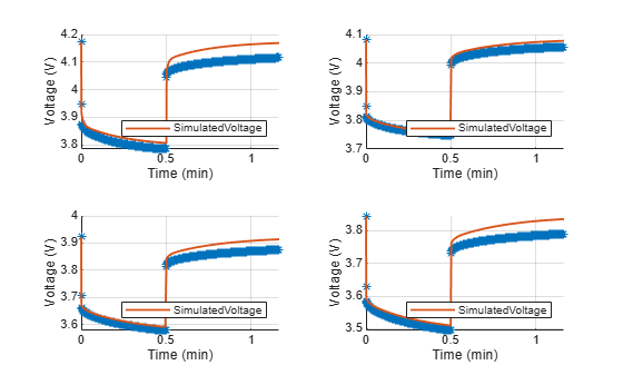
To verify the accuracy of the fit for each specific current pulse, use the plot function. The plot function optionally accepts a second argument that specifies the index of the pulse fit that you want to visualize. This index refers to the PulseID column inside the ParameterSummary property table. You can specify this index as a scalar or a vector.
Plot the fit for the first four discharge pulses.
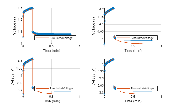
plot(batteryEcm,1:4)
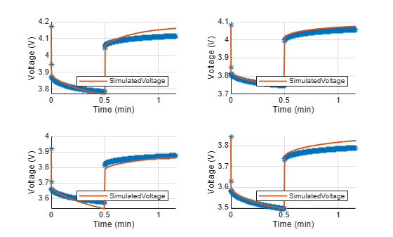
Plot the fit for the charge pulses 10, 11, 12, and 13.
plot(batteryEcm,10:13)
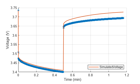
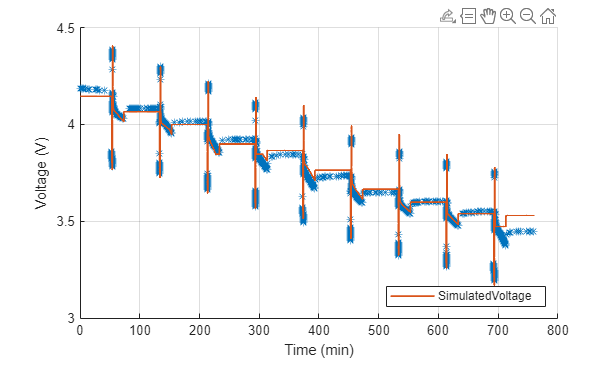
Once the you identify the ECM impedance parameters, to perform parameter verification, you can simulate the entire HPPCTest. The fitECM function only fits impedance and open-circuit voltage parameters in the data. If the test does not cover the full SOC range of a battery, the verification does not appear correct in these test areas.
To verify the resulting model against the HPPC test data, select only the portion of the test that contains the pulses.
data = hppcData((300:21475),:);
data.("time (s)") = data.("time (s)")-data.("time (s)")(1);
hppcExp25degCSim = hppcTest(data, ...
    TimeVariable="time (s)", ...
    VoltageVariable="voltage (V)", ...
    CurrentVariable="current (A)", ...
    Capacity=2.84, ...
    InitialSOC=1);
Visualize the model verification by using the simulateHPPCTest function.
simulateHPPCTest(batteryEcm,hppcExp25degCSim)
Alternatively, you can try different ECM topologies to achieve a better fit. Create an ECM object and specify the required number of parallel resistor-capacitor pairs.
battery3RCECM = ecm(3);
To estimate the model parameters for this ECM object, use the fitECM function.
battery3RCECM = fitECM(hppcExp25degC,ECM=battery3RCECM, ...
    SegmentToFit="loadAndRelaxation");
To verify the accuracy of the fit for each specific current pulse, use the plot function.
plot(battery3RCECM,1:4)
Single Resistor or Direct Current Internal Resistance (DCIR) Tables
The battery industry widely uses DCIR tables. Create an ECM object with no parallel resistor-capacitor pairs. This topology represents a single resistor.
batteryECMSingleRes = ecm(0);
Estimate the model parameters for this ECM by using the fitECM function.
batteryECMSingleRes = fitECM(hppcExp25degC,ECM=batteryECMSingleRes);
The ECM automatically populates with the DCIRs at different time frames depending on the pulse duration. The fitECM function uses these time frames: 2 seconds, 5 seconds, 10 seconds, 30 seconds, 60 seconds. For example, If the pulse duration is less than 60 seconds, the fitECM function does not include this DCIR value in the output table.
To view all the DCIR tables, use the TestParameterTables property of the batteryECMSingleRes object.
disp(batteryECMSingleRes.TestParameterTables)
                TestBreakpoints: [1×1 struct]
       ChargeOpenCircuitVoltage: [3.5098 3.5695 3.6224 3.6936 3.7905 3.8751 3.9674 4.0570 4.1158]
                   ChargeDCIR2s: [0.0482 0.0467 0.0461 0.0458 0.0460 0.0458 0.0461 0.0470 0.0513]
                   ChargeDCIR5s: [0.0507 0.0491 0.0483 0.0484 0.0490 0.0487 0.0490 0.0495 0.0545]
                       ChargeR0: [0.0507 0.0491 0.0483 0.0484 0.0490 0.0487 0.0490 0.0495 0.0545]
                    ChargeFitPc: [100 100 100 100 100 100 100 100 100]
    DischargeOpenCircuitVoltage: [3.5507 3.6015 3.6500 3.7353 3.8460 3.9226 4.0837 4.1745]
                DischargeDCIR2s: [0.0463 0.0448 0.0442 0.0450 0.0459 0.0456 0.0467 0.0525]
                DischargeDCIR5s: [0.0484 0.0467 0.0460 0.0470 0.0483 0.0480 0.0486 0.0552]
                    DischargeR0: [0.0484 0.0467 0.0460 0.0470 0.0483 0.0480 0.0486 0.0552]
                 DischargeFitPc: [100 100 100 100 100 100 100 100]
Estimate Parameters for Suite of HPPCTest Objects
You can perform battery HPPC testing at many different conditions, including temperature, SOC, current, and remaining capacity. You can then store these tests in more than one file. Simscape Battery refers to several HPPC test files as a HPPC test suite. HPPC test suites are typically categorized depending on the battery temperature at the start of each current pulse, which remains constant across different SOC values and load currents. In other cases, the initial temperature of the battery can also vary inside a given test file depending on the test settings and thermal environment.
In Simscape Battery, you can estimate multi-dimensional parameter tables for a suite of HPPC tests by merging different battery ECM objects or by using an hppcTestSuite object.
Merge Battery ECM Objects
You can perform parameter estimation for different HPPCTest objects at different temperatures, SOC values, or currents, and subsequently merge the resulting parameters into a single ECM object with a single set of multi-dimensional parameter tables. In this section, you estimate the ECM parameters for an HPPC test conducted at 0°C. First load the HPPC data.
load("testDataBAKcells/hppcDataBAKcell0degC.mat")Create the HPPCTest object by using the hppcTest function.
hppcExp0degC = hppcTest( hppcData,...
    TimeVariable="time (s)",...
    VoltageVariable="voltage (V)",...
    CurrentVariable="current (A)",...
    Temperature=zeros(numel(hppcData(:,1)),1));
Estimate the ECM parameters by using the fitECM function.
batteryECM0degC = fitECM(hppcExp0degC, ...
    SegmentToFit="loadAndRelaxation");
The batteryEcm object you created before represents the ECM at 25°C. You can add or merge the 0 °C HPPC test parameters to the 25 °C model by using the mergeModelParameters function.
batteryEcm = mergeModelParameters(batteryEcm,batteryECM0degC);
Visualize the test parameter tables of the merged model.
disp(batteryEcm.TestParameterTables)
                       TestBreakpoints: [1×1 struct]
       ChargeOpenCircuitVoltageThermal: [2×14 double]
                       ChargeR0Thermal: [2×14 double]
                       ChargeR1Thermal: [2×14 double]
                     ChargeTau1Thermal: [2×14 double]
                       ChargeC1Thermal: [2×14 double]
                       ChargeR2Thermal: [2×14 double]
                     ChargeTau2Thermal: [2×14 double]
                       ChargeC2Thermal: [2×14 double]
                    ChargeFitPcThermal: [2×14 double]
    DischargeOpenCircuitVoltageThermal: [2×15 double]
                    DischargeR0Thermal: [2×15 double]
                    DischargeR1Thermal: [2×15 double]
                  DischargeTau1Thermal: [2×15 double]
                    DischargeC1Thermal: [2×15 double]
                    DischargeR2Thermal: [2×15 double]
                  DischargeTau2Thermal: [2×15 double]
                    DischargeC2Thermal: [2×15 double]
                 DischargeFitPcThermal: [2×15 double]
Verify that the test breakpoints are 0°C and 25°C as expected.
disp(batteryEcm.TestParameterTables.TestBreakpoints.ResistanceTemperatureBreakpoints)
     0
    25
Inspect the ChargeR0Thermal parameter values of the TestParameterTables property.
disp(batteryEcm.TestParameterTables.ChargeR0Thermal)
    0.0496    0.0502    0.0509    0.0501    0.0510    0.0501    0.0500    0.0502    0.0507    0.0491    0.0501    0.0459    0.0490    0.0403
    0.0384    0.0383    0.0383    0.0383    0.0384    0.0384    0.0382    0.0385    0.0390    0.0390    0.0400    0.0400    0.0403    0.0403
Use HPPCTestSuite Objects
To estimate multi-dimensional parameter tables for a suite of HPPC tests, first load HPPC files for experiments conducted at 10 °C, 35 °C, and 45 °C, and then create different HPPCTest objects.
load("testDataBAKcells/hppcDataBAKcell10degC.mat")
hppcExp10degC = hppcTest(hppcData, ...
    TimeVariable="time (s)", ...
    VoltageVariable="voltage (V)", ...
    CurrentVariable="current (A)", ...
    Temperature=repmat(10,numel(hppcData(:,1)),1));
load("testDataBAKcells/hppcDataBAKcell35degC.mat")
hppcExp35degC = hppcTest(hppcData, ...
    TimeVariable="time (s)", ...
    VoltageVariable="voltage (V)", ...
    CurrentVariable="current (A)", ...
    Temperature=repmat(35,numel(hppcData(:,1)),1));
load("testDataBAKcells/hppcDataBAKcell45degC.mat")
hppcExp45degC = hppcTest(hppcData, ...
    TimeVariable="time (s)", ...
    VoltageVariable="voltage (V)", ...
    CurrentVariable="current (A)", ...
    Temperature=repmat(45,numel(hppcData(:,1)),1));
To create an HPPCTestSuite object, use the hppcTestSuite function.
hppcSuite = hppcTestSuite([hppcExp0degC;hppcExp10degC;hppcExp25degC;hppcExp35degC;hppcExp45degC], ...
    Temperature=[0;10;25;35;45]);
disp(hppcSuite.SuiteSummary)
TestID Test Temperature NumPulses
______ ________________________________________ ___________ _________
1 1×1 simscape.battery.parameters.HPPCTest 0 18
2 1×1 simscape.battery.parameters.HPPCTest 10 18
3 1×1 simscape.battery.parameters.HPPCTest 25 17
4 1×1 simscape.battery.parameters.HPPCTest 35 18
5 1×1 simscape.battery.parameters.HPPCTest 45 19
To estimate the model parameters for an HPPCTestSuite object with the default ECM, use the fitECM function.
batteryEcm = fitECM(hppcSuite);
The fitECM function estimates the parameters for each pulse and stores the resulting parameters in the TestParameterTables property.
disp(batteryEcm.TestParameterTables)
                       TestBreakpoints: [1×1 struct]
       ChargeOpenCircuitVoltageThermal: [5×25 double]
                       ChargeR0Thermal: [5×25 double]
                       ChargeR1Thermal: [5×25 double]
                     ChargeTau1Thermal: [5×25 double]
                       ChargeC1Thermal: [5×25 double]
                       ChargeR2Thermal: [5×25 double]
                     ChargeTau2Thermal: [5×25 double]
                       ChargeC2Thermal: [5×25 double]
                    ChargeFitPcThermal: [5×25 double]
    DischargeOpenCircuitVoltageThermal: [5×25 double]
                    DischargeR0Thermal: [5×25 double]
                    DischargeR1Thermal: [5×25 double]
                  DischargeTau1Thermal: [5×25 double]
                    DischargeC1Thermal: [5×25 double]
                    DischargeR2Thermal: [5×25 double]
                  DischargeTau2Thermal: [5×25 double]
                    DischargeC2Thermal: [5×25 double]
                 DischargeFitPcThermal: [5×25 double]
These parameter tables can be different to the final model parameters that you use in Simscape Battery. The difference resides in the breakpoint properties that you specify for the ECM object. View the ModelParameterTables properties.
disp(batteryEcm.ModelParameterTables)
       ChargeOpenCircuitVoltageThermal: [3×11 double]
                       ChargeR0Thermal: [3×11 double]
                       ChargeR1Thermal: [3×11 double]
                     ChargeTau1Thermal: [3×11 double]
                       ChargeC1Thermal: [3×11 double]
                       ChargeR2Thermal: [3×11 double]
                     ChargeTau2Thermal: [3×11 double]
                       ChargeC2Thermal: [3×11 double]
                    ChargeFitPcThermal: [3×11 double]
    DischargeOpenCircuitVoltageThermal: [3×11 double]
                    DischargeR0Thermal: [3×11 double]
                    DischargeR1Thermal: [3×11 double]
                  DischargeTau1Thermal: [3×11 double]
                    DischargeC1Thermal: [3×11 double]
                    DischargeR2Thermal: [3×11 double]
                  DischargeTau2Thermal: [3×11 double]
                    DischargeC2Thermal: [3×11 double]
                 DischargeFitPcThermal: [3×11 double]
You can manually change the resistance breakpoints by updating the ResistanceTemperatureBreakpoints property of the batteryECM object.
batteryEcm.ResistanceTemperatureBreakpoints = simscape.Value([0,10,25,35,45]+273.15,"K"); View the updated ModelParameterTables property.
disp(batteryEcm.ModelParameterTables)
       ChargeOpenCircuitVoltageThermal: [3×11 double]
                       ChargeR0Thermal: [5×11 double]
                       ChargeR1Thermal: [5×11 double]
                     ChargeTau1Thermal: [5×11 double]
                       ChargeC1Thermal: [5×11 double]
                       ChargeR2Thermal: [5×11 double]
                     ChargeTau2Thermal: [5×11 double]
                       ChargeC2Thermal: [5×11 double]
                    ChargeFitPcThermal: [5×11 double]
    DischargeOpenCircuitVoltageThermal: [3×11 double]
                    DischargeR0Thermal: [5×11 double]
                    DischargeR1Thermal: [5×11 double]
                  DischargeTau1Thermal: [5×11 double]
                    DischargeC1Thermal: [5×11 double]
                    DischargeR2Thermal: [5×11 double]
                  DischargeTau2Thermal: [5×11 double]
                    DischargeC2Thermal: [5×11 double]
                 DischargeFitPcThermal: [5×11 double]
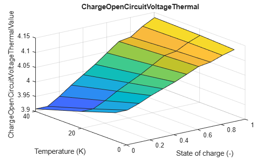
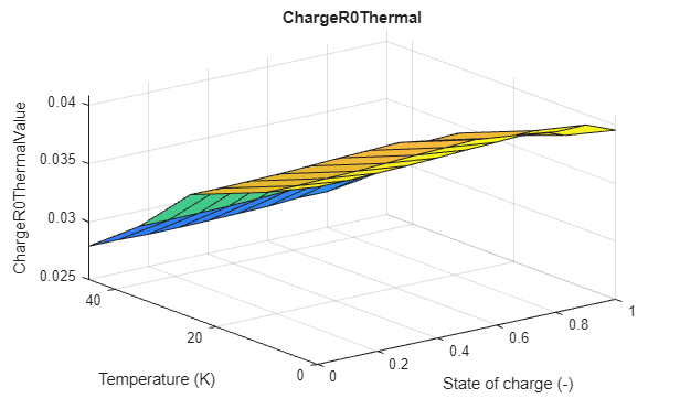
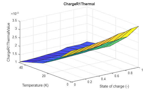
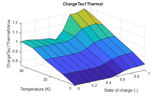
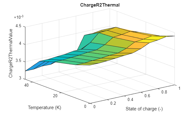
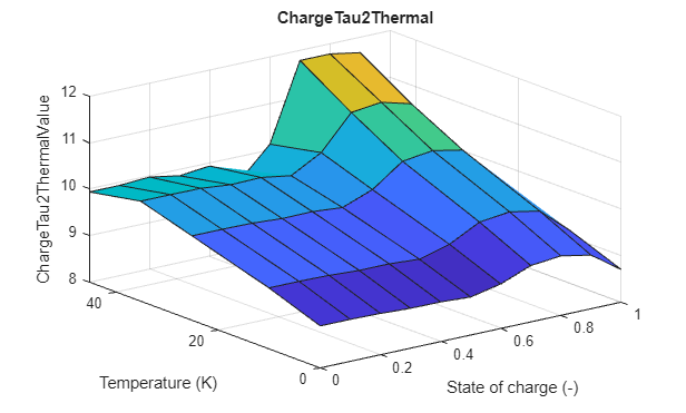
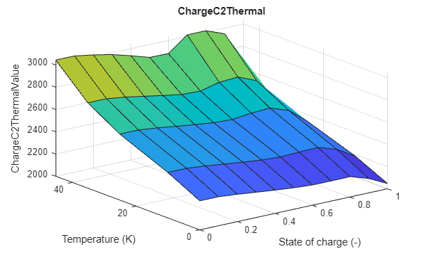
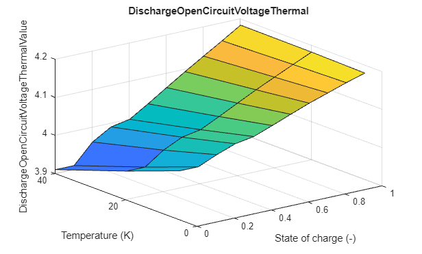
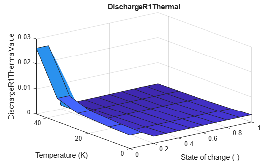
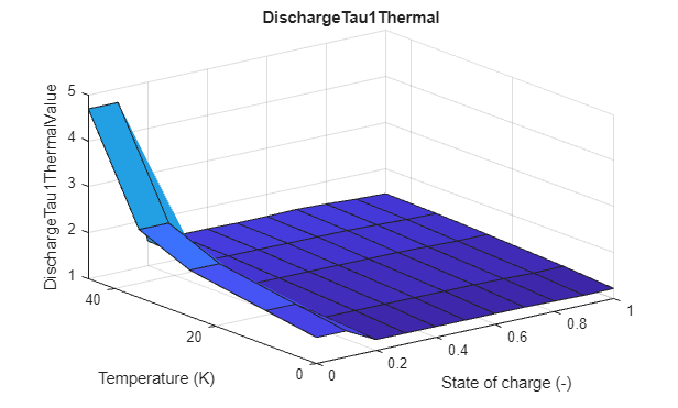
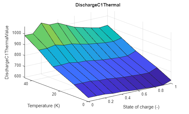
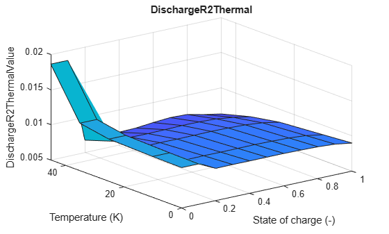
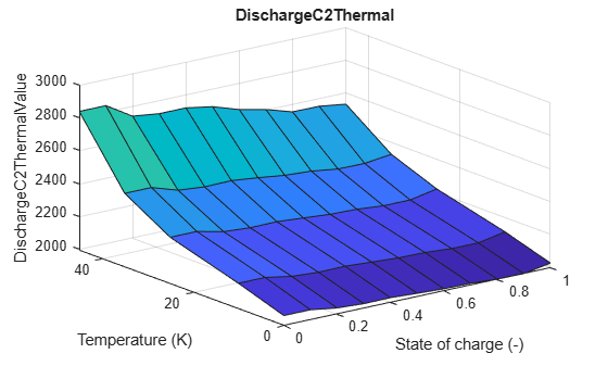
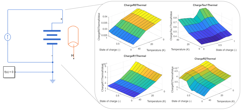
View the model parameters by using the plotModelParameters function.
batteryEcm.plotModelParameters();


Parameterize Battery Equivalent Circuit Block
You can parameterize the Battery Equivalent Circuit block as a final step in the parameterization workflow. This parameterization allows you to run battery simulations in Simulink®. To create a new Simulink battery model and add the Battery Equivalent Circuit block, use the createBatteryModel script.
if ~exist("batteryModel", 'file')
run("createBatteryModel.m")
end
Before parameterizing the block, you must obtain the block handle by using the getSimulinkBlockHandle function.
batteryBlockHandle = getSimulinkBlockHandle('batteryModel/Battery01');To automatically parameterize the Battery Equivalent Circuit block, use the parameterizeEquivalentCircuitBlock function.
batteryEcm.parameterizeEquivalentCircuitBlock(batteryBlockHandle,...
    ParameterizePseudoOCV=true)
Open the Battery Equivalent Circuit block mask to verify that the final model contains the correct parameter tables.
See Also
hppcTest | plot | removePulse | plotPulse | setChargeSOCs | setDischargeSOCs | ecm | fitECM | simulateHPPCTest | mergeModelParameters | plotModelParameters | hppcTestSuite | parameterizeEquivalentCircuitBlock | Battery Equivalent
Circuit