Estimate Battery Model Parameters from EIS Data

Since R2025a

This example shows how to estimate the model parameters for a battery equivalent circuit model (ECM) from electrochemical impedance spectroscopy (EIS) data using Simscape™ Battery™. The fractional-order equivalent circuit model (FOECM) is the ECM used for the analysis and interpretation of EIS data. EIS is a valuable technique that you can use to probe or investigate the impedance dynamics of electrochemical systems, such as batteries and fuel cells. Traditionally, during an EIS test, you apply a small, alternating current (AC) signal to an electrochemical cell and measure the resulting voltage response. This voltage response allows for the characterization of complex impedance over a range of frequencies at different operating conditions, including the initial battery soak temperature, initial state of charge (SOC), current or load, current directionality, state of health (SOH) or remaining capacity, and load frequency.

In this example, first you define the FOECM by creating an EISModel object in MATLAB®, which allows you to simulate and visualize the impedance of the FOECM in the frequency domain. Then, you estimate the parameters of the FOECM that best approximate a given EIS profile.

Simulate Frequency Response of FOECM

To represent an FOECM in MATLAB®, create an EISModel object by using the eisModel function.

eisfom = eisModel(); 
disp(eisfom)

  EISModel with properties:

     CircuitTopology: "R0+L1+(R1,CPE1)+(R2,CPE2)+CPE3"
       NumParameters: 10
       ParameterList: ["R0"    "L1"    "R1"    "CPE1n"    "CPE1Q"    "R2"    "CPE2n"    "CPE2Q"    "CPE3n"    "CPE3Q"]
     ParameterValues: [0.0250 1.0000e-06 0.0035 0.8000 1 0.0350 0.8000 10 0.8000 100]
    CircuitImpedance: "((((R0 + (i*w*L1)) + ((R1 * (1/(((i*w)^CPE1n)*CPE1Q))) / (R1 + (1/(((i*w)^CPE1n)*CPE1Q))))) + ((R2 * (1/(((i*w)^CPE2n)*CPE2Q))) / (R2 + (1/(((i*w)^CPE2n)*CPE2Q))))) + (1/(((i*w)^CPE3n)*CPE3Q)))"
       ParameterList: ["R0"    "L1"    "R1"    "CPE1n"    "CPE1Q"    "R2"    "CPE2n"    "CPE2Q"    "CPE3n"    "CPE3Q"]

Show all properties

This figure shows the equivalent circuit topology of the default EISModel object:

The EISModel object allows you to specify the type, amount, and connectivity of the electrical circuit elements that comprise the FOECM by using the CircuitTopology property. You define the circuit topology by using a string value. Use a "+" sign to represent a series connection. Use a "( , )" sign to represent a parallel connection. There is no limit to the amount of nested parallel or series connections.

This table shows the electrical circuit elements that the CircuitTopology property supports:

Name	Identifier String	Impedance	Mechanism
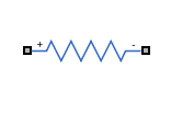
Resistor	R	$R$	Ohmic resistance of the electrolyte, electrodes, and other conductors.
Capacitor	C	$\frac{1}{j * w * C}$	Double layer at the electrode or electrolyte interface
Inductor	L	$j * w * L$	Inductive effects due to leads, conductors, and wiring in the measuring device
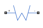
Constant Phase Element	CPE	$\frac{1}{{(j * w)}^{n} * Q}$	Accounts for non-deal capacitive behavior, often due to surface roughness, inhomogeneity, or porous electrodes.
Finite Space Warburg	FSW	$\frac{Z}{\sqrt{j * w * t}} * \coth (\sqrt{j * w * t})$	Diffusion processes that occur inside a finite region, for example within a solid-state battery electrolyte
Semi-Infinite Warburg	W	$\frac{W}{\sqrt{w}} * (1 - j)$	Diffusion processes in an unbounded medium, such as diffusion of redox species in the bulk electrolyte of a redox flow battery
Finite-Length Warburg	FLW	$\frac{Z}{\sqrt{j * w * t}} * \tanh (\sqrt{j * w * t})$	Diffusion processes in a medium with a defined length, for example in a thin-layer cell

Define the circuit topology of your EISModel object as a resistor in series with a parallel resistor-capacitor network.

eisfom.CircuitTopology = "R0+(R1,C1)";
disp(eisfom)

  EISModel with properties:

     CircuitTopology: "R0+(R1,C1)"
       NumParameters: 3
       ParameterList: ["R0"    "R1"    "C1"]
     ParameterValues: [0.0250 0.0035 150]
    CircuitImpedance: "(R0 + ((R1 * (1/(i*w*C1))) / (R1 + (1/(i*w*C1)))))"
       ParameterList: ["R0"    "R1"    "C1"]

Show all properties

To simulate the frequency model, define the frequency points you want to simulate the model at.

freq = logspace(-2,5,100);

Simulate the EIS circuit at these frequencies by using the simulateFrequencyResponse function. This function returns both the real and imaginary components of the impedance.

[simRealZ,simImagZ] = eisfom.simulateFrequencyResponse(freq);

Plot the frequency response on a Nyquist diagram by using the plot function. The impedance traces a semi-circular arc.

plot(simRealZ,-simImagZ,linewidth=1.5)
axis equal

Figure contains an axes object. The axes object contains an object of type line.

Now simulate the frequency response for a Warburg impedance. Set the CircuitTopology property of your EISModel object to "SIW1". The Warburg impedance is often used to model diffusion-controlled processes.

eisfom.CircuitTopology = "SIW1";
[simRealZ, simImagZ] = eisfom.simulateFrequencyResponse(freq);

Plot the frequency response. The plot shows the resulting impedances as a 45° line on the Nyquist diagram.

plot(simRealZ,-simImagZ,linewidth=1.5)
axis equal

Figure contains an axes object. The axes object contains an object of type line.

Integrate the previous circuit topology with the resistor and the RC pair. Set the CircuitTopology property of your EISModel object to "R0 + (R1,C1) + SIW1" and simulate the frequency response.

eisfom.CircuitTopology = "R0 + (R1,C1) + SIW1";
[simRealZ, simImagZ] = eisfom.simulateFrequencyResponse(freq);

Plot the frequency response on a Nyquist diagram. The Nyquist plot illustrates the influence of the R-RC circuit at high frequencies as a semicircle, and the influence of the Warburg impedance at low frequencies as a 45° line.

plot(simRealZ,-simImagZ,linewidth=1.5)
axis equal

Figure contains an axes object. The axes object contains an object of type line.

Estimate FOECM Parameters

By using the empirical EIS data, you can estimate the model parameters of the FOECM.

Load the EIS data. This data has been measured for a cell with a capacity of 5 Ah at a temperature of 25°C. This data consists of a 100-by-3 matrix of doubles. The columns of the matrix refer to the frequency, real impedance, and imaginary impedance values, respectively.

load("battery5Ah25degC.mat","data")

Fit the default EIS model to the measured data. To fit the data, use the fitEISModel function. The fitEISModel function returns an EISModel object.

eisfom = fitEISModel(data);

View the model circuit topology and the other properties.

disp(eisfom)

  EISModel with properties:

     CircuitTopology: "R0+L1+(R1,CPE1)+(R2,CPE2)+CPE3"
       NumParameters: 10
       ParameterList: ["R0"    "L1"    "R1"    "CPE1n"    "CPE1Q"    "R2"    "CPE2n"    "CPE2Q"    "CPE3n"    "CPE3Q"]
     ParameterValues: [0.0125 1.6255e-10 0.0086 1.0000 0.9434 0.0348 0.9952 12.6841 0.4613 372.6422]
    CircuitImpedance: "((((R0 + (i*w*L1)) + ((R1 * (1/(((i*w)^CPE1n)*CPE1Q))) / (R1 + (1/(((i*w)^CPE1n)*CPE1Q))))) + ((R2 * (1/(((i*w)^CPE2n)*CPE2Q))) / (R2 + (1/(((i*w)^CPE2n)*CPE2Q))))) + (1/(((i*w)^CPE3n)*CPE3Q)))"
       ParameterList: ["R0"    "L1"    "R1"    "CPE1n"    "CPE1Q"    "R2"    "CPE2n"    "CPE2Q"    "CPE3n"    "CPE3Q"]

Show all properties

Analyze how the function performed the fit on the frequency model by using the plot function. This plot shows the simulated data against the measured data, where the X-axis represents the real part of the impedance and the Y-axis represents the imaginary part of the impedance.

figure5Ah = uifigure(Name="Fitting Results 5 Ah Cell");
plot(eisfom,Parent=figure5Ah);

Figure Fitting Results 5 Ah Cell contains an object of type simscape.battery.parameters.ui.impedanceverificationchart.

Obtain Initial Estimates for Battery EIS Model

The fitEISModel function is heavily dependent on the initial parameter guess to perform the parameter fitting or optimization. Furthermore, the parameter values of different electrochemical systems can vary significantly due to numerous factors, such as temperature, size, and other variables. To obtain the initial estimates for the parameters of a battery EIS model, use the estimateBatteryEISParameters function. This function accepts different name-value arguments, including BatteryCapacity, BatteryTemperature, and BatteryRemainingCapacity. This function only returns the parameter estimates for the default EISModel object circuit topology.

initialParameters = estimateBatteryEISParameters(BatteryCapacity=simscape.Value(30/1000,"Ah"));

Fit the EIS model based on the initial parameters you estimated.

load("battery30mAh25degC.mat","data");
eisfom = fitEISModel(data,InitialParameterEstimate=initialParameters);

Analyze the accuracy of the fit by using the plot function.

figure30mAh = uifigure(Name="Fitting Results 30 mAh Cell")

figure30mAh = 
  Figure (Fitting Results 30 mAh Cell) with properties:

      Number: []
        Name: 'Fitting Results 30 mAh Cell'
       Color: [0.9608 0.9608 0.9608]
    Position: [348 367 583 437]
       Units: 'pixels'

  Show all properties

plot(eisfom,1,DisplayMode="Nyquist",Parent=figure30mAh);

Figure Fitting Results 30 mAh Cell contains an object of type simscape.battery.parameters.ui.impedanceverificationchart.

Estimate Battery Model Parameters from EIS Data

Simulate Frequency Response of FOECM

Estimate FOECM Parameters

Obtain Initial Estimates for Battery EIS Model

See Also

Topics