Main Content

plot

Plot HPPC test voltage over time

Since R2025a

Description

plot(myHppcTest) plots the entire hybrid pulse power characterization (HPPC) test voltage over time, showing the identified charge and discharge pulse indices.

plot(myHppcTest,Name=Value) plots the HPPC test voltage and specifies options using one or more name-value arguments.

example

chart = plot(___) returns a HPPCChart object.

Examples

collapse all

This example shows how to plot the entire hybrid pulse power characterization (HPPC) test voltage over time.

Open the DownloadBatteryData example and load the required HPPC data obtained for a BAK 2.9 Ah battery cell at 25 °C. This data consists of a table with three columns. The columns of the table refer to time, voltage, and current values, respectively.

openExample("simscapebattery/DownloadBatteryDataExample")
load("testDataBAKcells/hppcDataBAKcell25degC.mat")

Store the HPPC data inside an HPPCTest object by using the hppcTest function. You can use this object to view the data, add or edit breakpoints, add or remove pulses, and include additional information such as state of charge and capacity. The HPPC data is a table, so you must also specify each column name by using the TimeVariable, VoltageVariable, and CurrentVariable arguments. These names must match the names of the columns in the hppcData table.

hppcExp = hppcTest(hppcData,...
    TimeVariable="time (s)",...
    VoltageVariable="voltage (V)",...
    CurrentVariable="current (A)");

Analyze the TestSummary property of the hppcExp object. This property contains a summary of the HPPC test that shows all the identified pulses and related data, returned as a table.

hppcExp.TestSummary
ans =

  18×13 table

    PulseID    Directionality      SOC          HPPCData         PulseDuration    PseudoOCV_V    MaximumVoltage    MinimumVoltage    Current_A    C_rate    PulseStartIndex    PulseEndIndex    Temperature_degC
    _______    ______________    _______    _________________    _____________    ___________    ______________    ______________    _________    ______    _______________    _____________    ________________

       1        "Discharge"            1    {701×6 timetable}         30            4.1745           4.1745            3.7846         -6.1869     1.8976           354              1055               25       
       2        "Discharge"      0.90376    {701×6 timetable}         30            4.0837           4.0837            3.7479          -6.187     1.8977          2702              3403               25       
       3        "Discharge"      0.80754    {702×6 timetable}         30            4.0132           4.0132            3.6652         -6.1867     1.8975          5049              5751               25       
       4        "Discharge"      0.71133    {701×6 timetable}         30            3.9226           3.9226            3.5775         -6.1868     1.8976          7398              8099               25       
       5        "Discharge"      0.61512    {701×6 timetable}         30             3.846            3.846            3.4942         -6.1868     1.8976          9746             10447               25       
       6        "Discharge"      0.51891    {701×6 timetable}         30            3.7353           3.7353            3.4001         -6.1871     1.8977         12094             12795               25       
       7        "Discharge"       0.4227    {701×6 timetable}         30              3.65             3.65            3.3236         -6.1867     1.8975         14442             15143               25       
       8        "Discharge"      0.32649    {701×6 timetable}         30            3.6015           3.6015            3.2652         -6.1869     1.8976         16790             17491               25       
       9        "Discharge"      0.23028    {701×6 timetable}         30            3.5507           3.5507            3.1931         -6.1869     1.8976         19138             19839               25       
      10        "Charge"         0.98415    {502×6 timetable}         10            4.1158           4.3889            4.1158          4.6393      1.423          1055              1557               25       
      11        "Charge"         0.88793    {502×6 timetable}         10             4.057           4.3001             4.057          4.6406     1.4233          3403              3905               25       
      12        "Charge"         0.79172    {502×6 timetable}         10            3.9674           4.2113            3.9674          4.6394      1.423          5751              6253               25       
      13        "Charge"         0.69551    {502×6 timetable}         10            3.8751           4.1175            3.8751          4.6396      1.423          8099              8601               25       
      14        "Charge"          0.5993    {502×6 timetable}         10            3.7905           4.0355            3.7905          4.6396      1.423         10447             10949               25       
      15        "Charge"         0.50309    {502×6 timetable}         10            3.6936           3.9339            3.6936          4.6405     1.4233         12795             13297               25       
      16        "Charge"         0.40688    {502×6 timetable}         10            3.6224           3.8602            3.6224          4.6396      1.423         15143             15645               25       
      17        "Charge"         0.31066    {502×6 timetable}         10            3.5695           3.8109            3.5695          4.6397     1.4231         17491             17993               25       
      18        "Charge"         0.21445    {502×6 timetable}         10            3.5098           3.7597            3.5098          4.6397     1.4231         19839             20341               25    

Plot the entire HPPC test voltage using the plot function. You can specify optional name-value arguments, such as the parent container of the chart or the visibility of the charge and discharge pulse indices.

plot(hppcExp,Parent=figure);

Plot of the HPPC test voltage. The X axis represents time, in minutes. The Y axis represents the voltage, in volts. Orange circles in the plot represent the discharge indices. Orange stars in the plot represent the charge indices

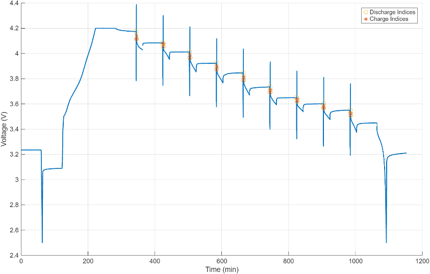
The plot shows all the identified charge and discharge pulse indices inside the TestSummary property table of the hppcExp object.

Input Arguments

collapse all

HPPC test container to plot, specified as an HPPCTest object.

Name-Value Arguments

expand all

Specify optional pairs of arguments as Name1=Value1,...,NameN=ValueN, where Name is the argument name and Value is the corresponding value. Name-value arguments must appear after other arguments, but the order of the pairs does not matter.

Example: plot(myTest,ChargePulseIndicesVisible="on")

Plot Arguments

expand all

Visibility of the charge pulse indices highlighted on the chart, specified as "off", "on", or as numeric or logical 1 (true) or 0 (false). A value of "on" is equivalent to true, and "off" is equivalent to false. Thus, you can use the value of this property as a logical value. The value is stored as an on/off logical value of type matlab.lang.OnOffSwitchState.

Visibility of the discharge pulse indices highlighted on the chart, specified as "off", "on", or as numeric or logical 1 (true) or 0 (false). A value of "on" is equivalent to true, and "off" is equivalent to false. Thus, you can use the value of this property as a logical value. The value is stored as an on/off logical value of type matlab.lang.OnOffSwitchState.

Visibility of the chart axes, specified as "off", "on", or as numeric or logical 1 (true) or 0 (false). A value of "on" is equivalent to true, and "off" is equivalent to false. Thus, you can use the value of this property as a logical value. The value is stored as an on/off logical value of type matlab.lang.OnOffSwitchState.

ChartContainer Arguments

expand all

Chart size and location, excluding the margins for decorations such as axis labels and tick marks. Specify this property as a vector of form [left bottom width height]. The values are in the units specified by the Units property.

  • left — Distance from the left edge of the parent container to the inner-left edge of the chart that excludes the margins. Typically, the parent container is a figure, panel, or tab.

  • bottom — Distance from the bottom edge of the parent container to the inner-bottom edge of the chart that excludes the margins.

  • width — Width of the chart, excluding the margins.

  • height — Height of the chart, excluding the margins.

Note

Setting this property has no effect when the parent of the chart is a TiledChartLayout.

Chart size and location, including the margins for decorations such as axis labels and tick marks. Specify this property as a vector of form [left bottom width height]. The values are in the units specified by the Units property.

  • left — Distance from the left edge of the parent container to the outer-left edge of the chart that includes the margins. Typically, the parent container is a figure, panel, or tab.

  • bottom — Distance from the bottom edge of the parent container to the outer-bottom edge of the chart that includes the margins.

  • width — Width of chart, including the margins.

  • height — Height of chart, including the margins.

Note

Setting this property has no effect when the parent of the chart is a TiledChartLayout.

Chart size and location, excluding the margins for decorations such as axis labels and tick marks. Specify this property as a vector of form [left bottom width height]. This property is equivalent to the InnerPosition property.

Note

Setting this property has no effect when the parent of the chart is a TiledChartLayout.

Position property to hold constant when adding, removing, or changing decorations, specified as one of the following values:

  • 'outerposition' — The OuterPosition property remains constant when you add, remove, or change decorations such as a title or an axis label. If any positional adjustments are needed, MATLAB® adjusts the InnerPosition property.

  • 'innerposition' — The InnerPosition property remains constant when you add, remove, or change decorations such as a title or an axis label. If any positional adjustments are needed, MATLAB adjusts the OuterPosition property.

Position units, specified as a value from the following table. To change the position of the chart in specific units, set the Units property before specifying the Position property. If you specify the Units and Position properties in a single command (using name-value pairs), be sure to specify Units before Position.

UnitsDescription
'normalized' (default)Normalized with respect to the parent container, which is typically the figure, panel, or tab. The lower left corner of the container maps to (0,0), and the upper right corner maps to (1,1).
'inches'Inches.
'centimeters'Centimeters.
'characters'

Based on the default font of the graphics root object:

  • Character width = width of letter x.

  • Character height = distance between the baselines of two lines of text.

'points'Typography points. One point equals 1/72 inch.
'pixels'

Pixels.

On Windows® and Macintosh systems, the size of a pixel is 1/96th of an inch. This size is independent of your system resolution.

On Linux® systems, the size of a pixel is determined by your system resolution.

Layout options, specified as a TiledChartLayoutOptions object. This property specifies options when an instance of your chart is a child of a tiled chart layout. If the instance is not a child of a tiled chart layout (for example, it is a child of a figure or panel), then this property is empty and has no effect. Otherwise, you can position the chart within the layout by setting the Tile and TileSpan properties on the TiledChartLayoutOptions object.

For example, this code places chart object c into the third tile of a tiled chart layout.

c.Layout.Tile = 3;

To make the chart span multiple tiles, specify the TileSpan property as a two-element vector. For example, this chart spans 2 rows and 3 columns of tiles.

c.Layout.TileSpan = [2 3];

Note

Tiled chart layouts are not supported for the axes returned by the getAxes method. Instead, you can place an instance of your chart into a tiled chart layout.

State of visibility, specified as 'on' or 'off', or as numeric or logical 1 (true) or 0 (false). A value of 'on' is equivalent to true, and 'off' is equivalent to false. Thus, you can use the value of this property as a logical value. The value is stored as an on/off logical value of type matlab.lang.OnOffSwitchState.

  • 'on' — Display the chart.

  • 'off' — Hide the chart without deleting it. You still can access the properties of chart when it is not visible.

Parent container of the chart, specified as a Figure, Panel, Tab, or TiledChartLayout object.

Visibility of the chart object handle in its parent's list of children, specified as one of these values:

  • 'on' — Chart object handle is always visible.

  • 'off' — Chart object handle is invisible at all times. This option is useful for preventing unintended changes to the chart by another function. To temporarily hide the handle during the execution of that function, set the HandleVisibility to 'off'.

  • 'callback' — Chart object handle is visible from within callbacks or functions invoked by callbacks, but not from within functions invoked from the command line. This option blocks access to the object in the Command Window, but it allows callback functions to access it.

If the object is not listed in the Children property of the chart's parent object, then functions that get object handles by searching the object hierarchy or querying handle properties cannot return it. This includes get, findobj, gca, gcf, gco, newplot, cla, clf, and close.

Hidden object handles are still valid. Set the root ShowHiddenHandles property to 'on' to list all object handles, regardless of their HandleVisibility property setting.

Output Arguments

collapse all

Chart for visualizing the identified discharge and charge pulses in a voltage plot, returned as a HPPCChart object.

Version History

Introduced in R2025a