islinphase

Determine whether filter has linear phase

Syntax

flag = islinphase(b,a)

flag = islinphase(B,A,"ctf")

flag = islinphase({B,A,g},"ctf")

flag = islinphase(d)

flag = islinphase(sos)

flag = islinphase(___,tol)

Description

flag = islinphase(b,a) returns a logical output equal to 1 if the specified filter is linear phase. Specify a filter with numerator coefficients b and denominator coefficients a.

flag = islinphase(B,A,"ctf") returns 1 if the filter specified as Cascaded Transfer Functions (CTF) with numerator coefficients B and denominator coefficients A is linear phase. (since R2024b)

flag = islinphase({B,A,g},"ctf") returns 1 if the filter specified in CTF format is linear phase. Specify the filter with numerator coefficients B, denominator coefficients A, and scaling values g across filter sections. (since R2024b)

flag = islinphase(d) returns 1 if the digital filter d is linear phase.

flag = islinphase(sos) returns 1 if the filter specified by the second-order sections matrix sos is linear phase.

flag = islinphase(___,tol) specifies a tolerance tol to determine when two numbers are close enough to be considered equal.

Examples

Linear and Nonlinear Phase Filters

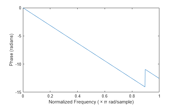
Use the window method to design a tenth-order lowpass FIR filter with normalized cutoff frequency 0.55. Verify that the filter has linear phase.

d = designfilt("lowpassfir",DesignMethod="window", ...
    FilterOrder=10,CutoffFrequency=0.55);
flag = islinphase(d)

flag = logical
   1

[phs,w] = phasez(d);

plot(w/pi,phs)
xlabel("Normalized Frequency (\times\pi rad/sample)")
ylabel("Phase (radians)")

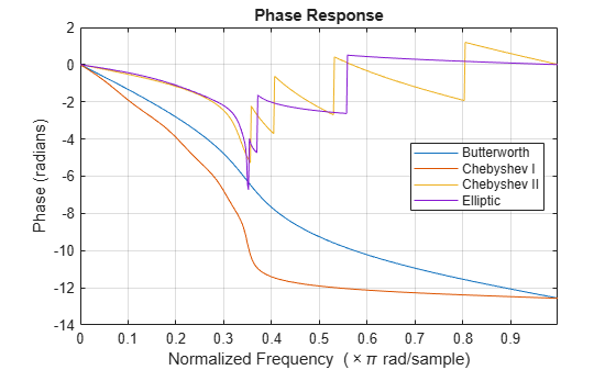
IIR filters in general do not have linear phase. Verify the statement by constructing eighth-order Butterworth, Chebyshev, and elliptic filters with similar specifications.

ord = 8;
Wcut = 0.35;
atten = 20;
rippl = 1;

[zb,pb,kb] = butter(ord,Wcut);
sosB = zp2sos(zb,pb,kb);

[zc,pc,kc] = cheby1(ord,rippl,Wcut);
sosC1 = zp2sos(zc,pc,kc);

[zd,pd,kd] = cheby2(ord,atten,Wcut);
sosC2 = zp2sos(zd,pd,kd);

[ze,pe,ke] = ellip(ord,rippl,atten,Wcut);
sosE = zp2sos(ze,pe,ke);

Plot the phase responses of the filters. Determine whether they have linear phase.

phasez(sosB)
hold on
phasez(sosC1)
phasez(sosC2)
phasez(sosE)
hold off
ylim([-14 2])
legend("Butterworth","Chebyshev I", ...
    "Chebyshev II","Elliptic",Location="best")

phs = [islinphase(sosB) islinphase(sosC1) ...
       islinphase(sosC2) islinphase(sosE)]

phs = 1×4 logical array

   0   0   0   0

Verify Linear Phase from Cascaded Transfer Functions

Since R2024b

Design a 40th-order lowpass Chebyshev type II digital filter with a stopband edge frequency of 0.4 and stopband attenuation of 50 dB. Verify that the filter has linear phase using the filter coefficients in the CTF format.

[B,A] = cheby2(40,50,0.4,"ctf");

flag = islinphase(B,A,"ctf")

flag = logical
   0

Design a 30th-order bandpass elliptic digital filter with passband edge frequencies of 0.3 and 0.7, passband ripple of 0.1 dB, and stopband attenuation of 50 dB. Verify that the filter has linear phase using the filter coefficients and gain in the CTF format.

[B,A,g] = ellip(30,0.1,50,[0.3 0.7],"ctf");
flag = islinphase({B,A,g},"ctf")

flag = logical
   0

Input Arguments

b,a — Transfer function coefficients

vector

Transfer function coefficients, specified as a vector. The values of b and a represent the numerator and denominator polynomial coefficients, respectively.

Example: [b,a] = cheby2(5,30,0.7) creates a digital 5th-order Butterworth lowpass filter with coefficients b and a, having a normalized 3 dB frequency of 0.7π rad/sample and 30 dB attenuation at stopband.

Data Types: single | double
Complex Number Support: Yes

B,A — Cascaded transfer function (CTF) coefficients

scalars | vectors | matrices

Since R2024b

Cascaded transfer function (CTF) coefficients, specified as scalars, vectors, or matrices. B and A list the numerator and denominator coefficients of the cascaded transfer function, respectively.

B must be of size L-by-(m + 1) and A must be of size L-by-(n + 1), where:

• L represents the number of filter sections.

• m represents the order of the filter numerators.

• n represents the order of the filter denominators.

For more information about the cascaded transfer function format and coefficient matrices, see Specify Digital Filters in CTF Format.

Note

If any element of A(:,1) is not equal to 1, then islinphase normalizes the filter coefficients by A(:,1). In this case, A(:,1) must be nonzero.

Data Types: double | single
Complex Number Support: Yes

g — Scale values

scalar | vector

Since R2024b

Scale values, specified as a real-valued scalar or as a real-valued vector with L + 1 elements, where L is the number of CTF sections. The scale values represent the distribution of the filter gain across sections of the cascaded filter representation.

The islinphase function applies a gain to the filter sections using the scaleFilterSections function depending on how you specify g:

• Scalar — The function distributes the gain uniformly across all filter sections.

• Vector — The function applies the first L gain values to the corresponding filter sections and distributes the last gain value uniformly across all filter sections.

Data Types: double | single

d — Digital filter

digitalFilter object

Digital filter, specified as a digitalFilter object. Use designfilt to generate d based on frequency-response specifications.

Example: designfilt("lowpassfir",FilterOrder=10,CutoffFrequency=0.55) generates a digitalFilter object for a 10th order FIR lowpass filter with a normalized 3 dB frequency of 0.55π rad/sample.

Data Types: digitalFilter

sos — Second-order section representation

L-by-6 matrix

Second-order section representation, specified as an L-by-6 matrix, where L is the number of second-order sections. The matrix

$$\text{sos}=\left[\begin{array}{cccccc}{b}_{01}& b_{11}& b_{21}& 1& a_{11}& a_{21}\\ b_{02}& b_{12}& b_{22}& 1& a_{12}& a_{22}\\ ⋮& ⋮& ⋮& ⋮& ⋮& ⋮\\ b_{0L}& b_{1L}& b_{2L}& 1& a_{1L}& a_{2L}\end{array}\right]$$

represents the second-order sections of H(z):

$$H(z)={\displaystyle \prod _{k=1}^L{H}_k(z)={\displaystyle \prod _{k=1}^L\frac{b_{0k}+b_{1k}{z}^{-1}+b_{2k}{z}^{-2}}{1+a_{1k}{z}^{-1}+a_{2k}{z}^{-2}}.}}$$

Example: [z,p,k] = butter(3,1/32); sos = zp2sos(z,p,k) specifies a third-order Butterworth filter with a normalized 3 dB frequency of π/32 rad/sample.

Data Types: single | double
Complex Number Support: Yes

tol — Tolerance

eps^(2/3) (default) | positive scalar

Tolerance to distinguish between close numbers, specified as a positive scalar. The tolerance value determines when two numbers are close enough to be considered equal.

Data Types: single | double

Output Arguments

flag — Linear phase flag

logical

Linear phase flag, returned as a logical scalar. The function returns 1 when the input is a minimum phase filter.

More About

Cascaded Transfer Functions

Partitioning an IIR digital filter into cascaded sections improves its numerical stability and reduces its susceptibility to coefficient quantization errors. The cascaded form of a transfer function H(z) in terms of the L transfer functions H₁(z), H₂(z), …, H_L(z) is

$$H(z)={\displaystyle \prod _{l=1}^L{H}_l(z)}=H_1(z)\times H_2(z)\times \cdots \times H_L(z).$$

Specify Digital Filters in CTF Format

You can specify digital filters in the CTF format for analysis, visualization, and signal filtering. Specify a filter by listing its coefficients B and A. You can also include the filter scaling gain across sections by specifying a scalar or vector g.

Filter Coefficients

When you specify the coefficients as L-row matrices,

$$B=\left[\begin{array}{cccc}{b}_{11}& b_{12}& \cdots & b_{1,m+1}\\ b_{21}& b_{22}& \cdots & b_{2,m+1}\\ ⋮& ⋮& \ddots & ⋮\\ b_{L1}& b_{L2}& \cdots & b_{L,m+1}\end{array}\right],A=\left[\begin{array}{cccc}{a}_{11}& a_{12}& \cdots & a_{1,n+1}\\ a_{21}& a_{22}& \cdots & a_{2,n+1}\\ ⋮& ⋮& \ddots & ⋮\\ a_{L1}& a_{L2}& \cdots & a_{L,n+1}\end{array}\right],$$

it is assumed that you have specified the filter as a sequence of L cascaded transfer functions, such that the full transfer function of the filter is

$$H\left(z\right)=\frac{b_{11}+b_{12}{z}^{-1}+\cdots +b_{1,m+1}{z}^{-m}}{a_{11}+a_{12}{z}^{-1}+\cdots +a_{1,n+1}{z}^{-n}}\times \frac{b_{21}+b_{22}{z}^{-1}+\cdots +b_{2,m+1}{z}^{-m}}{a_{21}+a_{22}{z}^{-1}+\cdots +a_{2,n+1}{z}^{-n}}\times \cdots \times \frac{b_{L1}+b_{L2}{z}^{-1}+\cdots +b_{L,m+1}{z}^{-m}}{a_{L1}+a_{L2}{z}^{-1}+\cdots +a_{L,n+1}{z}^{-n}},$$

where m ≥ 0 is the numerator order of the filter and n ≥ 0 is the denominator order.

• If you specify both B and A as vectors, it is assumed that the underlying system is a one-section IIR filter (L = 1), with B representing the numerator of the transfer function and A representing its denominator.

• If B is scalar, it is assumed that the filter is a cascade of all-pole IIR filters with each section having an overall system gain equal to B.

• If A is scalar, it is assumed that the filter is a cascade of FIR filters with each section having an overall system gain equal to 1/A.

Note

• To convert second-order section matrices to cascaded transfer functions, use the sos2ctf function.

• To convert a zero-pole-gain filter representation to cascaded transfer functions, use the zp2ctf function.

Coefficients and Gain

If you have an overall scaling gain or multiple scaling gains factored out from the coefficient values, you can specify the coefficients and gain as a cell array of the form {B,A,g}. Scaling filter sections is especially important when you work with fixed-point arithmetic to ensure that the output of each filter section has similar amplitude levels, which helps avoid inaccuracies in the filter response due to limited numeric precision.

The gain can be a scalar overall gain or a vector of section gains.

• If the gain is scalar, the value applies uniformly to all the cascade filter sections.

• If the gain is a vector, it must have one more element than the number of filter sections L in the cascade. Each of the first L scale values applies to the corresponding filter section, and the last value applies uniformly to all the cascade filter sections.

If you specify the coefficient matrices and gain vector as

$$B=\left[\begin{array}{cccc}{b}_{11}& b_{12}& \cdots & b_{1,m+1}\\ b_{21}& b_{22}& \cdots & b_{2,m+1}\\ ⋮& ⋮& \ddots & ⋮\\ b_{L1}& b_{L2}& \cdots & b_{L,m+1}\end{array}\right],A=\left[\begin{array}{cccc}{a}_{11}& a_{12}& \cdots & a_{1,n+1}\\ a_{21}& a_{22}& \cdots & a_{2,n+1}\\ ⋮& ⋮& \ddots & ⋮\\ a_{L1}& a_{L2}& \cdots & a_{L,n+1}\end{array}\right],g=\left[\begin{array}{ccccc}{g}_1& g_2& \cdots & g_L& g_{\text{S}}\end{array}\right],$$

it is assumed that the transfer function of the filter system is

$$H\left(z\right)=g_{\text{S}}\left(g_1\frac{b_{11}+b_{12}{z}^{-1}+\cdots +b_{1,m+1}{z}^{-m}}{a_{11}+a_{12}{z}^{-1}+\cdots +a_{1,n+1}{z}^{-n}}\times g_2\frac{b_{21}+b_{22}{z}^{-1}+\cdots +b_{2,m+1}{z}^{-m}}{a_{21}+a_{22}{z}^{-1}+\cdots +a_{2,n+1}{z}^{-n}}\times \cdots \times g_L\frac{b_{L1}+b_{L2}{z}^{-1}+\cdots +b_{L,m+1}{z}^{-m}}{a_{L1}+a_{L2}{z}^{-1}+\cdots +a_{L,n+1}{z}^{-n}}\right).$$

Tips

• You can obtain filters in CTF format, including the scaling gain. Use the outputs of digital IIR filter design functions, such as butter, cheby1, cheby2, and ellip. Specify the "ctf" filter-type argument in these functions and specify to return B, A, and g to get the scale values. (since R2024b)

References

[1] Lyons, Richard G. Understanding Digital Signal Processing. Upper Saddle River, NJ: Prentice Hall, 2004.

Version History

Introduced in R2013a

R2024b: Analyze filters using cascaded transfer functions

The islinphase function supports inputs in the cascaded transfer function (CTF) format.