Main Content

filter

Forward recursion of state-space models

Description

filter computes state-distribution moments for each period of the specified response data by recursively applying the Kalman filter.

To compute updated state-distribution moments efficiently during only the final period of the specified response data by applying one recursion of the Kalman filter, use update instead.

example

X = filter(Mdl,Y) returns filtered states (X) from performing forward recursion of the fully specified state-space model Mdl. That is, filter applies the standard Kalman filter using Mdl and the observed responses Y.

example

X = filter(Mdl,Y,Name,Value) uses additional options specified by one or more Name,Value arguments. For example, specify the regression coefficients and predictor data to deflate the observations, or specify to use the square-root filter.

If Mdl is not fully specified, then you must specify the unknown parameters as known scalars using the 'Params' Name,Value argument.

[X,logL,Output] = filter(___) uses any of the input arguments in the previous syntaxes to additionally return the loglikelihood value (logL) and an output structure array (Output) using any of the input arguments in the previous syntaxes. Output contains:

Examples

collapse all

Suppose that a latent process is an AR(1). The state equation is

xt=0.5xt-1+ut,

where ut is Gaussian with mean 0 and standard deviation 1.

Generate a random series of 100 observations from xt, assuming that the series starts at 1.5.

T = 100;
ARMdl = arima('AR',0.5,'Constant',0,'Variance',1);
x0 = 1.5;
rng(1); % For reproducibility
x = simulate(ARMdl,T,'Y0',x0);

Suppose further that the latent process is subject to additive measurement error. The observation equation is

yt=xt+εt,

where εt is Gaussian with mean 0 and standard deviation 0.75. Together, the latent process and observation equations compose a state-space model.

Use the random latent state process (x) and the observation equation to generate observations.

y = x + 0.75*randn(T,1);

Specify the four coefficient matrices.

A = 0.5;
B = 1;
C = 1;
D = 0.75;

Specify the state-space model using the coefficient matrices.

Mdl = ssm(A,B,C,D)
Mdl = 
State-space model type: ssm

State vector length: 1
Observation vector length: 1
State disturbance vector length: 1
Observation innovation vector length: 1
Sample size supported by model: Unlimited

State variables: x1, x2,...
State disturbances: u1, u2,...
Observation series: y1, y2,...
Observation innovations: e1, e2,...

State equation:
x1(t) = (0.50)x1(t-1) + u1(t)

Observation equation:
y1(t) = x1(t) + (0.75)e1(t)

Initial state distribution:

Initial state means
 x1 
  0 

Initial state covariance matrix
     x1   
 x1  1.33 

State types
     x1     
 Stationary 

Mdl is an ssm model. Verify that the model is correctly specified using the display in the Command Window. The software infers that the state process is stationary. Subsequently, the software sets the initial state mean and covariance to the mean and variance of the stationary distribution of an AR(1) model.

Filter states for periods 1 through 100. Plot the true state values and the filtered state estimates.

filteredX = filter(Mdl,y);

figure
plot(1:T,x,'-k',1:T,filteredX,':r','LineWidth',2)
title({'State Values'})
xlabel('Period')
ylabel('State')
legend({'True state values','Filtered state values'})

Figure contains an axes object. The axes object with title State Values, xlabel Period, ylabel State contains 2 objects of type line. These objects represent True state values, Filtered state values.

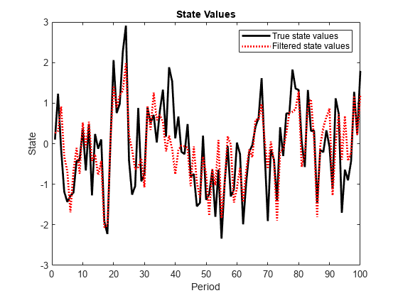
The true values and filter estimates are approximately the same.

Suppose that the linear relationship between the change in the unemployment rate and the nominal gross national product (nGNP) growth rate is of interest. Suppose further that the first difference of the unemployment rate is an ARMA(1,1) series. Symbolically, and in state-space form, the model is

[x1,tx2,t]=[ϕθ00][x1,t-1x2,t-1]+[11]u1,tyt-βZt=x1,t+σεt,

where:

  • x1,t is the change in the unemployment rate at time t.

  • x2,t is a dummy state for the MA(1) effect.

  • y1,t is the observed change in the unemployment rate being deflated by the growth rate of nGNP (Zt).

  • u1,t is the Gaussian series of state disturbances having mean 0 and standard deviation 1.

  • εt is the Gaussian series of observation innovations having mean 0 and standard deviation σ.

Load the Nelson-Plosser data set, which contains the unemployment rate and nGNP series, among other things.

load Data_NelsonPlosser

Preprocess the data by taking the natural logarithm of the nGNP series, and the first difference of each series. Also, remove the starting NaN values from each series.

isNaN = any(ismissing(DataTable),2);       % Flag periods containing NaNs
gnpn = DataTable.GNPN(~isNaN);
u = DataTable.UR(~isNaN);
T = size(gnpn,1);                          % Sample size
Z = [ones(T-1,1) diff(log(gnpn))];
y = diff(u);

Though this example removes missing values, the software can accommodate series containing missing values in the Kalman filter framework.

Specify the coefficient matrices.

A = [NaN NaN; 0 0];
B = [1; 1];
C = [1 0];
D = NaN;

Specify the state-space model using ssm.

Mdl = ssm(A,B,C,D);

Estimate the model parameters, and use a random set of initial parameter values for optimization. Specify the regression component and its initial value for optimization using the 'Predictors' and 'Beta0' name-value pair arguments, respectively. Restrict the estimate of σ to all positive, real numbers.

params0 = [0.3 0.2 0.2];
[EstMdl,estParams] = estimate(Mdl,y,params0,'Predictors',Z,...
    'Beta0',[0.1 0.2],'lb',[-Inf,-Inf,0,-Inf,-Inf]);
Method: Maximum likelihood (fmincon)
Sample size: 61
Logarithmic  likelihood:     -99.7245
Akaike   info criterion:      209.449
Bayesian info criterion:      220.003
           |      Coeff       Std Err    t Stat     Prob  
----------------------------------------------------------
 c(1)      |  -0.34098       0.29608    -1.15164  0.24948 
 c(2)      |   1.05003       0.41377     2.53771  0.01116 
 c(3)      |   0.48592       0.36790     1.32079  0.18657 
 y <- z(1) |   1.36121       0.22338     6.09358   0      
 y <- z(2) | -24.46711       1.60018   -15.29024   0      
           |                                              
           |    Final State   Std Dev     t Stat    Prob  
 x(1)      |   1.01264       0.44690     2.26592  0.02346 
 x(2)      |   0.77718       0.58917     1.31912  0.18713 

EstMdl is an ssm model, and you can access its properties using dot notation.

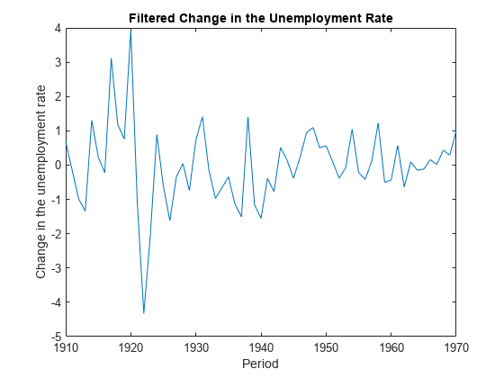
Filter the estimated state-space model. EstMdl does not store the data or the regression coefficients, so you must pass in them in using the name-value pair arguments 'Predictors' and 'Beta', respectively. Plot the estimated, filtered states. Recall that the first state is the change in the unemployment rate, and the second state helps build the first.

filteredX = filter(EstMdl,y,'Predictors',Z,'Beta',estParams(end-1:end));

figure
plot(dates(end-(T-1)+1:end),filteredX(:,1));
xlabel('Period')
ylabel('Change in the unemployment rate')
title('Filtered Change in the Unemployment Rate')

Figure contains an axes object. The axes object with title Filtered Change in the Unemployment Rate, xlabel Period, ylabel Change in the unemployment rate contains an object of type line.

Consider nowcasting the model in Filter States of Time-Invariant State-Space Model.

Generate a random series of 100 observations from xt.

T = 100;
A = 0.5;
B = 1;
C = 1;
D = 0.75;
Mdl = ssm(A,B,C,D);
rng(1); % For reproducibility
y = simulate(Mdl,T);

Suppose the final 10 observations are in the forecast horizon.

fh = 10;
yf = y((end-fh+1):end); % Holdout sample responses
y = y(1:end-fh);        % In-sample responses

Filter the observations through the model to obtain filtered states for each period.

[xhat,logL,output] = filter(Mdl,y);
xhatvar = output.FilteredStatesCov;

xhat and xhatvar are 90-by-1 vectors of in-sample filtered states and corresponding variances, respectively. xhat(t) is the estimate of E(xt|y1,...,yt), and xhatvar is the estimate of Var(xt|y1,...,yt).

Call filter again, but specify the real-time update option.

[xhatRT,logLRT,outputRT] = filter(Mdl,y,'RealTimeUpdate',true);
xhatRTvar = outputRT.FilteredStatesCov;

xhatRT and xhatRTvar are scalars representing the estimate of E(x90|y1,...,y90) and its corresponding variance, respectively.

Compare the filtered states and variances of period 90.

tol = 1e-10;
areMeansEqual = (xhat(end) - xhatRT) < tol
areMeansEqual = logical
   1

areVarsEqual = (xhatvar(end) - xhatRTvar) < tol
areVarsEqual = logical
   0

areLogLsEqual = (logL - logLRT) < tol;

In the last period, the filtered states, their variances, and the loglikelihoods are equal.

Nowcast the model into the forecast horizon by performing this procedure for each successive period:

  1. Set the initial state and its variance to their current filter estimates. This action changes the state-space model.

  2. As an observation becomes available, filter it through the model in real time.

% Initialize state and variance
state0 = xhatRT;        
var0 = xhatRTvar;

% Preallocate
xhatRTF = zeros(fh,1);
xhatRTvarF = zeros(fh,1);

for j = 1:fh
    Mdl.Mean0 = state0;
    Mdl.Cov0 = var0;
    [xhatRTF(j),~,outputRT] = filter(Mdl,yf(j),'RealTimeUpdate',true); % Alternatively, use update
    xhatRTvarF(j) = outputRT.FilteredStatesCov;
    state0 = xhatRTF(j);
    var0 = xhatRTvarF(j);
end

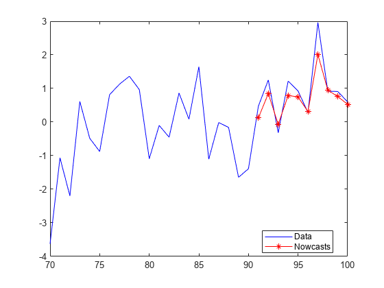
Plot the data and nowcasts.

figure
plot((T-fh-20):T,[y(end-20:end); yf],'b-',(T-fh+1):T,xhatRTF,'r*-')
legend(["Data" "Nowcasts"],'Location',"best")

Figure contains an axes object. The axes object contains 2 objects of type line. These objects represent Data, Nowcasts.

Input Arguments

collapse all

Standard state-space model, specified as an ssm model object returned by ssm or estimate.

If Mdl is not fully specified (that is, Mdl contains unknown parameters), then specify values for the unknown parameters using the 'Params' name-value argument. Otherwise, the software issues an error. estimate returns fully-specified state-space models.

Mdl does not store observed responses or predictor data. Supply the data wherever necessary using the appropriate input or name-value arguments.

Observed response data, specified as a numeric matrix or a cell vector of numeric vectors.

  • If Mdl is time invariant with respect to the observation equation, then Y is a T-by-n matrix, where each row corresponds to a period and each column corresponds to a particular observation in the model. T is the sample size and m is the number of observations per period. The last row of Y contains the latest observations.

  • If Mdl is time varying with respect to the observation equation, then Y is a T-by-1 cell vector. Each element of the cell vector corresponds to a period and contains an nt-dimensional vector of observations for that period. The corresponding dimensions of the coefficient matrices in Mdl.C{t} and Mdl.D{t} must be consistent with the matrix in Y{t} for all periods. The last cell of Y contains the latest observations.

NaN elements indicate missing observations. For details on how the Kalman filter accommodates missing observations, see Algorithms.

Name-Value Arguments

Specify optional pairs of arguments as Name1=Value1,...,NameN=ValueN, where Name is the argument name and Value is the corresponding value. Name-value arguments must appear after other arguments, but the order of the pairs does not matter.

Before R2021a, use commas to separate each name and value, and enclose Name in quotes.

Example: 'Beta',beta,'Predictors',Z specifies to deflate the observations by the regression component composed of the predictor data Z and the coefficient matrix beta.

Regression coefficients corresponding to predictor variables, specified as the comma-separated pair consisting of 'Beta' and a d-by-n numeric matrix. d is the number of predictor variables (see Predictors) and n is the number of observed response series (see Y).

If Mdl is an estimated state-space model, then specify the estimated regression coefficients stored in estParams.

Values for unknown parameters in the state-space model, specified as the comma-separated pair consisting of 'Params' and a numeric vector.

The elements of Params correspond to the unknown parameters in the state-space model matrices A, B, C, and D, and, optionally, the initial state mean Mean0 and covariance matrix Cov0.

  • If you created Mdl explicitly (that is, by specifying the matrices without a parameter-to-matrix mapping function), then the software maps the elements of Params to NaNs in the state-space model matrices and initial state values. The software searches for NaNs column-wise following the order A, B, C, D, Mean0, and Cov0.

  • If you created Mdl implicitly (that is, by specifying the matrices with a parameter-to-matrix mapping function), then you must set initial parameter values for the state-space model matrices, initial state values, and state types within the parameter-to-matrix mapping function.

If Mdl contains unknown parameters, then you must specify their values. Otherwise, the software ignores the value of Params.

Data Types: double

Predictor variables in the state-space model observation equation, specified as the comma-separated pair consisting of 'Predictors' and a T-by-d numeric matrix. T is the number of periods and d is the number of predictor variables. Row t corresponds to the observed predictors at period t (Zt). The expanded observation equation is

ytZtβ=Cxt+Dut.

That is, the software deflates the observations using the regression component. β is the time-invariant vector of regression coefficients that the software estimates with all other parameters.

If there are n observations per period, then the software regresses all predictor series onto each observation.

If you specify Predictors, then Mdl must be time invariant. Otherwise, the software returns an error.

By default, the software excludes a regression component from the state-space model.

Data Types: double

Square root filter method flag, specified as the comma-separated pair consisting of 'SquareRoot' and true or false. If true, then filter applies the square root filter method when implementing the Kalman filter.

If you suspect that the eigenvalues of the filtered state or forecasted observation covariance matrices are close to zero, then specify 'SquareRoot',true. The square root filter is robust to numerical issues arising from finite the precision of calculations, but requires more computational resources.

Example: 'SquareRoot',true

Data Types: logical

Forecast uncertainty threshold, specified as the comma-separated pair consisting of 'Tolerance' and a nonnegative scalar.

If the forecast uncertainty for a particular observation is less than Tolerance during numerical estimation, then the software removes the uncertainty corresponding to the observation from the forecast covariance matrix before its inversion.

It is best practice to set Tolerance to a small number, for example, le-15, to overcome numerical obstacles during estimation.

Example: 'Tolerance',le-15

Data Types: double

Univariate treatment of a multivariate series flag, specified as the comma-separated pair consisting of 'Univariate' and true or false. Univariate treatment of a multivariate series is also known as sequential filtering.

The univariate treatment can accelerate and improve numerical stability of the Kalman filter. However, all observation innovations must be uncorrelated. That is, DtDt' must be diagonal, where Dt, t = 1,...,T, is one of the following:

  • The matrix D{t} in a time-varying state-space model

  • The matrix D in a time-invariant state-space model

Example: 'Univariate',true

Data Types: logical

Flag indicating whether to apply the real-time filter, specified as a value in the table.

ValueDescription
true

filter returns only the final state distribution, which is the filtered state at time T (one forward recursion of the Kalman filter). Specifically, filter performs the following actions:

  1. Dispatch the model, data, and other specifications to the update function to update state distribution and compute the loglikelihood.

  2. Return only the final state distribution; outputs do not contain intermediate state distributions.

    • X is a 1-by-m vector of the final filtered states.

    • logL is a scalar of the sum of the loglikelihood.

    • Output is a 1-by-1 structure array associated with the recursion at time T. The fields include:

      • LogLikelihood: sum of the loglikelihood

      • FilteredStates: m-by-1 vector of filtered states

      • FilteredStatesCov: m-by-m uncertainty matrix of filtered states

Mdl must represent a standard state-space model (ssm object).

false

filter returns filtered states and results for each period in the input data Y.

Example: 'RealTimeUpdate',true

Data Types: logical

Output Arguments

collapse all

Filtered states, returned as a numeric matrix or a cell vector of numeric vectors.

If Mdl is time invariant, then the number of rows of X is the sample size, T, and the number of columns of X is the number of states, m. The last row of X contains the latest filtered states.

If Mdl is time varying, then X is a cell vector with length equal to the sample size. Cell t of X contains a vector of filtered states with length equal to the number of states in period t. The last cell of X contains the latest filtered states.

If you set the RealTimeUpdate name-value argument to true, filter returns only the filtered state for time T, a 1-by-m vector. For more details, see RealTimeUpdate.

Loglikelihood function value, returned as a scalar.

Missing observations do not contribute to the loglikelihood.

Filtering results by period, returned as a structure array.

Output is a T-by-1 structure, where element t corresponds to the filtering result at time t.

  • If Univariate is false (it is by default), then the following table outlines the fields of Output.

    FieldDescriptionEstimate of
    LogLikelihoodScalar loglikelihood objective function valueN/A
    FilteredStatesmt-by-1 vector of filtered statesE(xt|y1,...,yt)
    FilteredStatesCovmt-by-mt variance-covariance matrix of filtered statesVar(xt|y1,...,yt)
    ForecastedStatesmt-by-1 vector of state forecastsE(xt|y1,...,yt1)
    ForecastedStatesCovmt-by-mt variance-covariance matrix of state forecastsVar(xt|y1,...,yt1)
    ForecastedObsht-by-1 forecasted observation vectorE(yt|y1,...,yt1)
    ForecastedObsCovht-by-ht variance-covariance matrix of forecasted observationsVar(yt|y1,...,tt1)
    KalmanGainmt-by-nt adjusted Kalman gain matrixN/A
    DataUsedht-by-1 logical vector indicating whether the software filters using a particular observation. For example, if observation i at time t is a NaN, then element i in DataUsed at time t is 0.N/A

  • If Univarite is true, then the fields of Output are the same as in the previous table, except for the following amendments.

    FieldChanges
    ForecastedObsSame dimensions as if Univariate = 0, but only the first elements are equal
    ForecastedObsCov

    n-by-1 vector of forecasted observation variances.

    The first element of this vector is equivalent to ForecastedObsCov(1,1) when Univariate is false. The rest of the elements are not necessarily equivalent to their corresponding values in ForecastObsCov when Univariate.

    KalmanGainSame dimensions as if Univariate is false, though KalmanGain might have different entries.

If you set the RealTimeUpdate name-value argument to true, filter returns only the filtered states for time T, its covariance matrix, and the loglikelihood (in other words, the sum of the loglikelihoods returned by update). For more details, see RealTimeUpdate.

Tips

  • Mdl does not store the response data, predictor data, and the regression coefficients. Supply the data wherever necessary using the appropriate input or name-value arguments.

  • To accelerate estimation for low-dimensional, time-invariant models, set 'Univariate',true. Using this specification, the software sequentially updates rather then updating all at once during the filtering process.

Algorithms

  • The Kalman filter accommodates missing data by not updating filtered state estimates corresponding to missing observations. In other words, suppose there is a missing observation at period t. Then, the state forecast for period t based on the previous t – 1 observations and filtered state for period t are equivalent.

  • For explicitly defined state-space models, filter applies all predictors to each response series. However, each response series has its own set of regression coefficients.

Alternative Functionality

To filter a standard state-space model in real time by performing one forward recursion of the Kalman filter, call the update function instead. Unlike filter, update performs minimal input validation for computational efficiency.

References

[1] Durbin, J, and Siem Jan Koopman. Time Series Analysis by State Space Methods. 2nd ed. Oxford: Oxford University Press, 2012.

Version History

Introduced in R2014a