Test Open-Loop ADAS Algorithm Using Driving Scenario

This example shows how to test an open-loop ADAS (advanced driver assistance system) algorithm in Simulink®. In an open-loop ADAS algorithm, the ego vehicle behavior is predefined and does not change as the scenario advances during simulation.

To test the algorithm, you use a driving scenario that was saved from the Driving Scenario Designer app. In this example, you read in a scenario by using a Scenario Reader block, and then visualize the scenario and sensor detections on the Bird's-Eye Scope.

Inspect Driving Scenario

This example uses a driving scenario that is based on one of the prebuilt scenarios that you access through the Driving Scenario Designer app. For more details on these scenarios, see Prebuilt Driving Scenarios in Driving Scenario Designer.

Open the scenario file in the app.

drivingScenarioDesigner('LeftTurnScenario.mat')

To simulate the scenario, click Run. In this scenario, the ego vehicle travels north and goes straight through an intersection. A vehicle coming from the left side of the intersection turns left and ends up in front of the ego vehicle.

The ego vehicle has these sensors:

• A front-facing radar for generating object detections

• A front-facing camera and rear-facing camera for generating object and lane boundary detections

• A lidar on the center of its roof for generating point cloud data of the scenario

• Two ultrasonic sensors facing front-left and front-right for generating object detections

Inspect Model

The model in this example was generated from the app by selecting Export > Export Simulink Model. In the model, a Scenario Reader block reads the actors and roads from the scenario file and outputs the non-ego actors and lane boundaries. Open the model.

open_system('OpenLoopWithScenarios.slx')

In the Scenario Reader block, the Driving Scenario Designer file name parameter specifies the name of the scenario file. You can specify a scenario file that is on the MATLAB® search path, such as the scenario file used in this example, or the full path to a scenario file. Alternatively, you can specify a drivingScenario object by setting Source of driving scenario to From workspace, and then setting MATLAB or model workspace variable name to the name of a valid drivingScenario object workspace variable.

The Scenario Reader block outputs the poses of the non-ego actors in the scenario and the left-lane and right-lane boundaries of the ego vehicle. To output all lane boundaries of the road on which the ego vehicle is traveling, select the corresponding option for the Lane boundaries to output parameter.

The actors, lane boundaries, and ego vehicle pose are passed to a subsystem containing the sensor blocks. Open the subsystem.

open_system('OpenLoopWithScenarios/Detection Generators')

The Driving Radar Data Generator, Vision Detection Generator, Lidar Point Cloud Generator, and Ultrasonic Detection Generator blocks produce synthetic detections from the scenario. You can fuse this sensor data to generate tracks, such as in the open-loop example Sensor Fusion Using Synthetic Radar and Vision Data in Simulink.

The outputs of the sensor blocks in this model are in vehicle coordinates, where:

• The X-axis points forward from the ego vehicle.

• The Y-axis points to the left of the ego vehicle.

• The origin is located at the center of the rear axle of the ego vehicle.

Because this model is open loop, the ego vehicle behavior does not change as the simulation advances. Therefore, the Source of ego vehicle parameter is set to Scenario, and the block reads the predefined ego vehicle pose and trajectory from the scenario file. For vehicle controllers and other closed-loop models, set the Source of ego vehicle parameter to Input port. With this option, you specify an ego vehicle that is defined in the model as an input to the Scenario Reader block. For an example, see Test Closed-Loop ADAS Algorithm Using Driving Scenario.

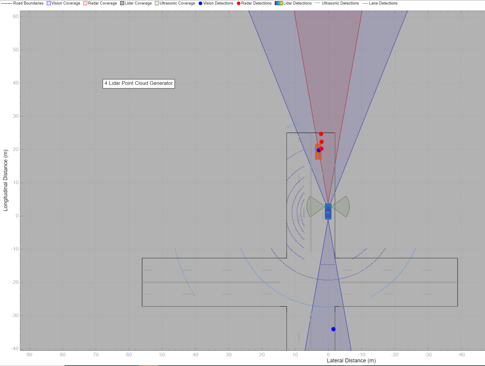
Visualize Simulation

To visualize the scenario and sensor detections, use the Bird's-Eye Scope. On the Simulink toolstrip, under Review Results, click Bird's-Eye Scope. Then, in the scope, click Find Signals and run the simulation.

Update Simulation Settings

This model uses the default simulation stop time of 10 seconds. Because the scenario is only about 5 seconds long, the simulation continues to run in the Bird's-Eye Scope even after the scenario has ended. To synchronize the simulation and scenario stop times, on the Simulink model toolbar, set the simulation stop time to 5.2 seconds, which is the exact stop time of the app scenario. After you run the simulation, the app displays this value in the bottom-right corner of the scenario canvas.

If the simulation runs too fast in the Bird's-Eye Scope, you can slow down the simulation by using simulation pacing. On the Simulink toolstrip, select Run > Simulation Pacing. Select the Enable pacing to slow down simulation check box and decrease the simulation time to slightly less than 1 second per wall-clock second, such as 0.8 seconds. Then, rerun the simulation in the Bird's-Eye Scope.