Quantify Image Quality Using Neural Image Assessment

This example uses:

This example shows how to analyze the aesthetic quality of images using a Neural Image Assessment (NIMA) convolutional neural network (CNN).

Image quality metrics provide an objective measure of image quality. An effective metric provides quantitative scores that correlate well with a subjective perception of quality by a human observer. Quality metrics enable the comparison of image processing algorithms.

NIMA [1] is a no-reference technique that predicts the quality of an image without relying on a pristine reference image, which is frequently unavailable. NIMA uses a CNN to predict a distribution of quality scores for each image.

Evaluate Image Quality Using Trained NIMA Model

Set dataDir as the desired location of the data set.

dataDir = fullfile(tempdir,"LIVEInTheWild");
if ~exist(dataDir,"dir")
    mkdir(dataDir);
end

Download a pretrained NIMA neural network by using the helper function downloadTrainedNetwork. The helper function is attached to the example as a supporting file. This model predicts a distribution of quality scores for each image in the range [1, 10], where 1 and 10 are the lowest and the highest possible values for the score, respectively. A high score indicates good image quality.

trainedNet_url = "https://ssd.mathworks.com/supportfiles/image/data/trainedNIMA.zip";
downloadTrainedNetwork(trainedNet_url,dataDir);
load(fullfile(dataDir,"trainedNIMA.mat"));

You can evaluate the effectiveness of the NIMA model by comparing the predicted scores for a high-quality and lower quality image.

Read a high-quality image into the workspace.

imOriginal = imread("kobi.png");

Reduce the aesthetic quality of the image by applying a Gaussian blur. Display the original image and the blurred image in a montage. Subjectively, the aesthetic quality of the blurred image is worse than the quality of the original image.

imBlur = imgaussfilt(imOriginal,5);
montage({imOriginal,imBlur})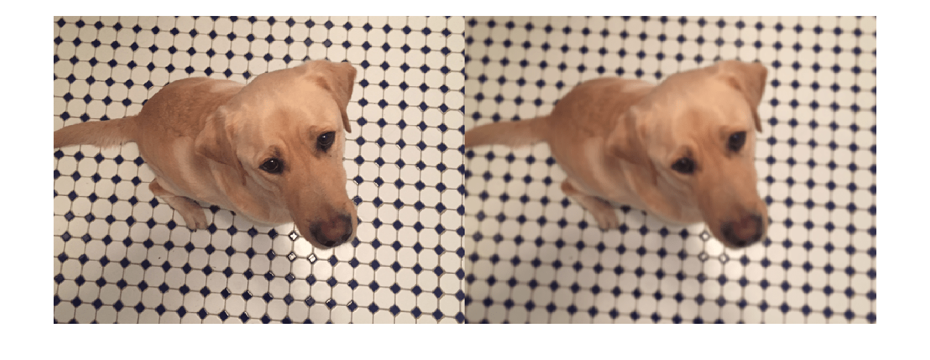

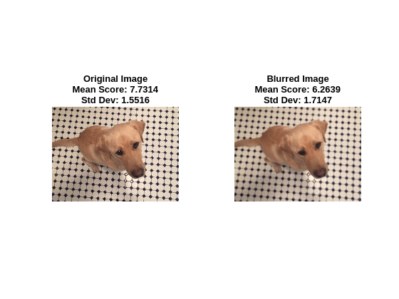
Predict the NIMA quality score distribution for the two images using the predictNIMAScore helper function. This function is attached to the example as a supporting file.

The predictNIMAScore function returns the mean and standard deviation of the NIMA score distribution for an image. The predicted mean score is a measure of the quality of the image. The standard deviation of scores can be considered a measure of the confidence level of the predicted mean score.

[meanOriginal,stdOriginal] = predictNIMAScore(dlnet,imOriginal);
[meanBlur,stdBlur] = predictNIMAScore(dlnet,imBlur);

Display the images along with the mean and standard deviation of the score distributions predicted by the NIMA model. The NIMA model correctly predicts scores for these images that agree with the subjective visual assessment.

figure
t = tiledlayout(1,2);
displayImageAndScoresForNIMA(t,imOriginal,meanOriginal,stdOriginal,"Original Image")
displayImageAndScoresForNIMA(t,imBlur,meanBlur,stdBlur,"Blurred Image")

The rest of this example shows how to train and evaluate a NIMA model.

Download LIVE In the Wild Data Set

This example uses the LIVE In the Wild data set [2], which is a public-domain subjective image quality challenge database. The data set contains 1162 photos captured by mobile devices, with 7 additional images provided to train the human scorers. Each image is rated by an average of 175 individuals on a scale of [1, 100]. The data set provides the mean and standard deviation of the subjective scores for each image.

Download the data set by following the instructions outlined in LIVE In the Wild Image Quality Challenge Database. Extract the data into the directory specified by the dataDir variable. When extraction is successful, dataDir contains two directories: Data and Images.

Load LIVE In the Wild Data

Get the file paths to the images.

imageData = load(fullfile(dataDir,"Data","AllImages_release.mat"));
imageData = imageData.AllImages_release;
nImg = length(imageData);
imageList(1:7) = fullfile(dataDir,"Images","trainingImages",imageData(1:7));
imageList(8:nImg) = fullfile(dataDir,"Images",imageData(8:end));

Create an image datastore that manages the image data.

imds = imageDatastore(imageList);

Load the mean and standard deviation data corresponding to the images.

meanData = load(fullfile(dataDir,"Data","AllMOS_release.mat"));
meanData = meanData.AllMOS_release;
stdData = load(fullfile(dataDir,"Data","AllStdDev_release.mat"));
stdData = stdData.AllStdDev_release;

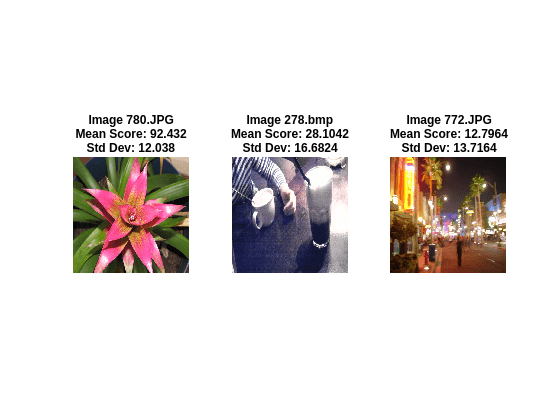
Optionally, display a few sample images from the data set with the corresponding mean and standard deviation values.

figure
t = tiledlayout(1,3);
idx1 = 785;
displayImageAndScoresForNIMA(t,readimage(imds,idx1), ...
    meanData(idx1),stdData(idx1),"Image "+imageData(idx1))
idx2 = 203;
displayImageAndScoresForNIMA(t,readimage(imds,idx2), ...
    meanData(idx2),stdData(idx2),"Image "+imageData(idx2))
idx3 = 777;
displayImageAndScoresForNIMA(t,readimage(imds,idx3), ...
    meanData(idx3),stdData(idx3),"Image "+imageData(idx3))

Preprocess and Augment Data

Preprocess the images by resizing them to 256-by-256 pixels.

rescaleSize = [256 256];
imds = transform(imds,@(x)imresize(x,rescaleSize));

The NIMA model requires a distribution of human scores, but the LIVE data set provides only the mean and standard deviation of the distribution. Approximate an underlying distribution for each image in the LIVE data set using the createNIMAScoreDistribution helper function. This function is attached to the example as a supporting file.

The createNIMAScoreDistribution rescales the scores to the range [1, 10], then generates maximum entropy distribution of scores from the mean and standard deviation values.

newMaxScore = 10;
prob = createNIMAScoreDistribution(meanData,stdData);
cumProb = cumsum(prob,2);

Create an arrayDatastore that manages the score distributions.

probDS = arrayDatastore(cumProb',IterationDimension=2);

Combine the datastores containing the image data and score distribution data.

dsCombined = combine(imds,probDS);

Preview the output of reading from the combined datastore.

sampleRead = preview(dsCombined)

sampleRead=1×2 cell array
    {256×256×3 uint8}    {10×1 double}

figure
tiledlayout(1,2)
nexttile
imshow(sampleRead{1})
title("Sample Image from Data Set")
nexttile
plot(sampleRead{2})
title("Cumulative Score Distribution")

Split Data for Training, Validation, and Testing

Partition the data into training, validation, and test sets. Allocate 70% of the data for training, 15% for validation, and the remainder for testing.

numTrain = floor(0.70 * nImg);
numVal = floor(0.15 * nImg);

Idx = randperm(nImg);
idxTrain = Idx(1:numTrain);
idxVal = Idx(numTrain+1:numTrain+numVal);
idxTest = Idx(numTrain+numVal+1:nImg);

dsTrain = subset(dsCombined,idxTrain);
dsVal = subset(dsCombined,idxVal);
dsTest = subset(dsCombined,idxTest);

Augment Training Data

Augment the training data using the augmentDataForNIMA helper function. This function is attached to the example as a supporting file. The augmentDataForNIMA function performs these augmentation operations on each training image:

Crop the image to 224-by-244 pixels to reduce overfitting.
Flip the image horizontally with 50% probability.

inputSize = [224 224];
dsTrain = transform(dsTrain,@(x)augmentDataForNIMA(x,inputSize));

Calculate Training Set Statistics for Input Normalization

The input layer of the network performs z-score normalization of the training images. Calculate the mean and standard deviation of the training images for use in z-score normalization.

meanImage = zeros([inputSize 3]);
meanImageSq = zeros([inputSize 3]);
while hasdata(dsTrain)
    dat = read(dsTrain);
    img = double(dat{1});
    meanImage = meanImage + img;
    meanImageSq = meanImageSq + img.^2;
end
meanImage = meanImage/numTrain;
meanImageSq = meanImageSq/numTrain;
varImage = meanImageSq - meanImage.^2;
stdImage = sqrt(varImage);

Reset the datastore to its initial state.

reset(dsTrain);

Batch Training Data

Create a minibatchqueue object that manages the mini-batching of observations in a custom training loop. The minibatchqueue object also casts data to a dlarray object that enables automatic differentiation in deep learning applications.

Specify the mini-batch data extraction format as "SSCB" (spatial, spatial, channel, batch). Set the "DispatchInBackground" name-value argument to the boolean returned by canUseGPU. If a supported GPU is available for computation, then the minibatchqueue object preprocesses mini-batches in the background in a parallel pool during training.

miniBatchSize = 128;
mbqTrain = minibatchqueue(dsTrain,MiniBatchSize=miniBatchSize, ...
    PartialMiniBatch="discard",MiniBatchFormat=["SSCB",""], ...
    DispatchInBackground=canUseGPU);
mbqVal = minibatchqueue(dsVal,MiniBatchSize=miniBatchSize, ...
    MiniBatchFormat=["SSCB",""],DispatchInBackground=canUseGPU);

Load and Modify MobileNet-v2 Network

This example starts with a MobileNet-v2 [3] CNN trained on ImageNet [4]. The example modifies the network by replacing the last layer of the MobileNet-v2 network with a fully connected layer with 10 neurons, each representing a discrete score from 1 through 10. The network predicts the probability of each score for each image. The example normalizes the outputs of the fully connected layer using a softmax activation layer.

The mobilenetv2 function returns a pretrained MobileNet-v2 network. This function requires the Deep Learning Toolbox™ Model for MobileNet-v2 Network support package. If this support package is not installed, then the function provides a download link.

net = mobilenetv2;

Convert the network into a layerGraph object.

lgraph = layerGraph(net);

The network has an image input size of 224-by-224 pixels. Replace the input layer with an image input layer that performs z-score normalization on the image data using the mean and standard deviation of the training images.

inLayer = imageInputLayer([inputSize 3],Name="input", ...
    Normalization="zscore",Mean=meanImage,StandardDeviation=stdImage);
lgraph = replaceLayer(lgraph,"input_1",inLayer);

Replace the original final classification layer with a fully connected layer with 10 neurons. Add a softmax layer to normalize the outputs. Set the learning rate of the fully connected layer to 10 times the learning rate of the baseline CNN layers. Apply a dropout of 75%.

lgraph = removeLayers(lgraph,["ClassificationLayer_Logits","Logits_softmax","Logits"]);
newFinalLayers = [
    dropoutLayer(0.75,Name="drop")
    fullyConnectedLayer(newMaxScore,Name="fc",WeightLearnRateFactor=10,BiasLearnRateFactor=10)
    softmaxLayer(Name="prob")];    
lgraph = addLayers(lgraph,newFinalLayers);
lgraph = connectLayers(lgraph,"global_average_pooling2d_1","drop");
dlnet = dlnetwork(lgraph);

Visualize the network using the Deep Network Designer app.

deepNetworkDesigner(lgraph)

Define Model Gradients and Loss Functions

The modelGradients helper function calculates the gradients and losses for each iteration of training the network. This function is defined in the Supporting Functions section of this example.

The objective of the NIMA network is to minimize the earth mover's distance (EMD) between the ground truth and predicted score distributions. EMD loss considers the distance between classes when penalizing misclassification. Therefore, EMD loss performs better than a typical softmax cross-entropy loss used in classification tasks [5]. This example calculates the EMD loss using the earthMoverDistance helper function, which is defined in the Supporting Functions section of this example.

For the EMD loss function, use an r-norm distance with r = 2. This distance allows for easy optimization when you work with gradient descent.

Specify Training Options

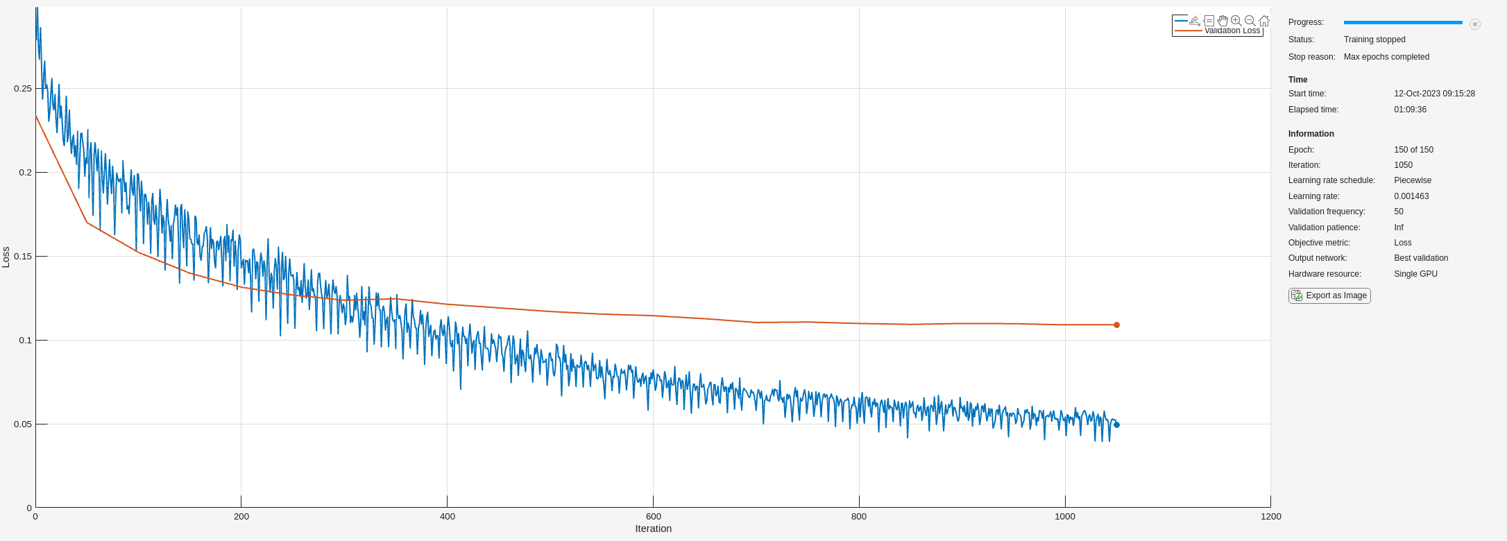
Specify the options for SGDM optimization. Train the network for 150 epochs.

numEpochs = 150;
momentum = 0.9;
initialLearnRate = 3e-3;
decay = 0.95;

Train Network

By default, the example loads a pretrained version of the NIMA network. The pretrained network enables you to run the entire example without waiting for training to complete.

To train the network, set the doTraining variable in the following code to true. Train the model in a custom training loop. For each iteration:

Read the data for the current mini-batch using the next function.
Evaluate the model gradients using the dlfeval function and the modelGradients helper function.
Update the network parameters using the sgdmupdate function.

Train on a GPU if one is available. Using a GPU requires Parallel Computing Toolbox™ and a CUDA® enabled NVIDIA® GPU. For more information, see GPU Computing Requirements (Parallel Computing Toolbox).

doTraining = false;
if doTraining
    iteration = 0;
    velocity = [];
    start = tic;
    
    [hFig,lineLossTrain,lineLossVal] = initializeTrainingPlotNIMA;
    
    for epoch = 1:numEpochs
        
        shuffle (mbqTrain);    
        learnRate = initialLearnRate/(1+decay*floor(epoch/10));
        
        while hasdata(mbqTrain)
            iteration = iteration + 1;        
            [dlX,cdfY] = next(mbqTrain);
            [grad,loss] = dlfeval(@modelGradients,dlnet,dlX,cdfY);        
            [dlnet,velocity] = sgdmupdate(dlnet,grad,velocity,learnRate,momentum);
            
            updateTrainingPlotNIMA(lineLossTrain,loss,epoch,iteration,start)              
        end
        
        % Add validation data to plot
        [~,lossVal,~] = modelPredictions(dlnet,mbqVal);
        updateTrainingPlotNIMA(lineLossVal,lossVal,epoch,iteration,start) 
        
    end
    
    % Save the trained network
    modelDateTime = string(datetime("now",Format="yyyy-MM-dd-HH-mm-ss"));
    save(fullfile(dataDir,"trainedNIMA-"+modelDateTime+".mat"),"dlnet");

else
    load(fullfile(dataDir,"trainedNIMA.mat"));    
end

Evaluate NIMA Model

Evaluate the performance of the model on the test data set using three metrics: EMD, binary classification accuracy, and correlation coefficients. The performance of the NIMA network on the test data set is in agreement with the performance of the reference NIMA model reported by Talebi and Milanfar [1].

Create a minibatchqueue object that manages the mini-batching of test data.

mbqTest = minibatchqueue(dsTest,MiniBatchSize=miniBatchSize,MiniBatchFormat=["SSCB",""]);

Calculate the predicted probabilities and ground truth cumulative probabilities of mini-batches of test data using the modelPredictions function. This function is defined in the Supporting Functions section of this example.

[YPredTest,~,cdfYTest] = modelPredictions(dlnet,mbqTest);

Calculate the mean and standard deviation values of the ground truth and predicted distributions.

meanPred = extractdata(YPredTest)' * (1:10)';
stdPred = sqrt(extractdata(YPredTest)'*((1:10).^2)' - meanPred.^2);
origCdf = extractdata(cdfYTest);
origPdf = [origCdf(1,:); diff(origCdf)];
meanOrig = origPdf' * (1:10)';
stdOrig = sqrt(origPdf'*((1:10).^2)' - meanOrig.^2);

Calculate EMD

Calculate the EMD of the ground truth and predicted score distributions. For prediction, use an r-norm distance with r = 1. The EMD value indicates the closeness of the predicted and ground truth rating distributions.

EMDTest = earthMoverDistance(YPredTest,cdfYTest,1)

EMDTest = 
  1×1 single gpuArray dlarray

    0.0974

Calculate Binary Classification Accuracy

For binary classification accuracy, convert the distributions to two classifications: high-quality and low-quality. Classify images with a mean score greater than a threshold as high-quality.

qualityThreshold = 5;
binaryPred = meanPred > qualityThreshold;    
binaryOrig = meanOrig > qualityThreshold;

Calculate the binary classification accuracy.

binaryAccuracy = 100 * sum(binaryPred==binaryOrig)/length(binaryPred)

binaryAccuracy =

   81.8182

Calculate Correlation Coefficients

Large correlation values indicate a large positive correlation between the ground truth and predicted scores. Calculate the linear correlation coefficient (LCC) and Spearman’s rank correlation coefficient (SRCC) for the mean scores.

meanLCC = corr(meanOrig,meanPred)

meanLCC =

  gpuArray single

    0.8270

meanSRCC = corr(meanOrig,meanPred,type="Spearman")

meanSRCC =

  gpuArray single

    0.8133

Supporting Functions

Model Gradients Function

The modelGradients function takes as input a dlnetwork object dlnet and a mini-batch of input data dlX with corresponding target cumulative probabilities cdfY. The function returns the gradients of the loss with respect to the learnable parameters in dlnet as well as the loss. To compute the gradients automatically, use the dlgradient function.

function [gradients,loss] = modelGradients(dlnet,dlX,cdfY)
    dlYPred = forward(dlnet,dlX);    
    loss = earthMoverDistance(dlYPred,cdfY,2);    
    gradients = dlgradient(loss,dlnet.Learnables);    
end

Loss Function

The earthMoverDistance function calculates the EMD between the ground truth and predicted distributions for a specified r-norm value. The earthMoverDistance uses the computeCDF helper function to calculate the cumulative probabilities of the predicted distribution.

function loss = earthMoverDistance(YPred,cdfY,r)
    N = size(cdfY,1);
    cdfYPred = computeCDF(YPred);
    cdfDiff = (1/N) * (abs(cdfY - cdfYPred).^r);
    lossArray = sum(cdfDiff,1).^(1/r);
    loss = mean(lossArray);
    
end
function cdfY = computeCDF(Y)
% Given a probability mass function Y, compute the cumulative probabilities
    [N,miniBatchSize] = size(Y);
    L = repmat(triu(ones(N)),1,1,miniBatchSize);
    L3d = permute(L,[1 3 2]);
    prod = Y.*L3d;
    prodSum = sum(prod,1);
    cdfY = reshape(prodSum(:)',miniBatchSize,N)';
end

Model Predictions Function

The modelPredictions function calculates the estimated probabilities, loss, and ground truth cumulative probabilities of mini-batches of data.

function [dlYPred,loss,cdfYOrig] = modelPredictions(dlnet,mbq)
    reset(mbq);
    loss = 0;
    numObservations = 0;
    dlYPred = [];    
    cdfYOrig = [];
    
    while hasdata(mbq)     
        [dlX,cdfY] = next(mbq);
        miniBatchSize = size(dlX,4);
        
        dlY = predict(dlnet,dlX);
        loss = loss + earthMoverDistance(dlY,cdfY,2)*miniBatchSize;
        dlYPred = [dlYPred dlY];
        cdfYOrig = [cdfYOrig cdfY];
        
        numObservations = numObservations + miniBatchSize;
        
    end
    loss = loss / numObservations;
end

References

[1] Talebi, Hossein, and Peyman Milanfar. “NIMA: Neural Image Assessment.” IEEE Transactions on Image Processing 27, no. 8 (August 2018): 3998–4011. https://doi.org/10.1109/TIP.2018.2831899.

[2] LIVE: Laboratory for Image and Video Engineering. "LIVE In the Wild Image Quality Challenge Database." https://live.ece.utexas.edu/research/ChallengeDB/index.html.

[3] Sandler, Mark, Andrew Howard, Menglong Zhu, Andrey Zhmoginov, and Liang-Chieh Chen. “MobileNetV2: Inverted Residuals and Linear Bottlenecks.” In 2018 IEEE/CVF Conference on Computer Vision and Pattern Recognition, 4510–20. Salt Lake City, UT: IEEE, 2018. https://doi.org/10.1109/CVPR.2018.00474.

[4] ImageNet. https://www.image-net.org.

[5] Hou, Le, Chen-Ping Yu, and Dimitris Samaras. “Squared Earth Mover’s Distance-Based Loss for Training Deep Neural Networks.” Preprint, submitted November 30, 2016. https://arxiv.org/abs/1611.05916.