estim
Form state estimator given estimator gain
Syntax
est = estim(sys,L)

est = estim(sys,L,sensors,known)
Description
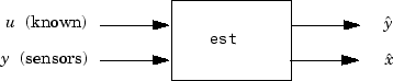
est = estim(sys,L) produces
a state/output estimator est given the plant state-space
model sys and the estimator gain L.
All inputs w of sys are assumed
stochastic (process and/or measurement noise), and all outputs y are
measured. The estimator est is returned in state-space
form (SS object).
For a continuous-time plant sys with equations
estim uses the following equations to generate
a plant output estimate and a state estimate , which are estimates
of y(t)=C and x(t),
respectively:
For a discrete-time plant sys with the following
equations:
estim uses estimator equations similar to
those for continuous-time to generate a plant output estimate and a state estimate , which are estimates
of y[n] and x[n],
respectively. These estimates are based on past measurements up to y[n-1].
est = estim(sys,L,sensors,known)
handles more general plants sys with both known
(deterministic) inputs u and stochastic inputs w,
and both measured outputs y and nonmeasured outputs z.
The index vectors sensors and known specify
which outputs of sys are measured (y),
and which inputs of sys are known (u).
The resulting estimator est, found using the following
equations, uses both u and y to
produce the output and state estimates.
Examples
Consider a state-space model sys with seven
outputs and four inputs. Suppose you designed a Kalman gain matrix L using
outputs 4, 7, and 1 of the plant as sensor measurements and inputs
1, 4, and 3 of the plant as known (deterministic) inputs. You can
then form the Kalman estimator by
sensors = [4,7,1];
known = [1,4,3];
est = estim(sys,L,sensors,known)
See the function kalman for
direct Kalman estimator design.
Tips
You can use the functions place (pole placement)
or kalman (Kalman filtering) to design an adequate
estimator gain L. Note that the estimator poles
(eigenvalues of A-LC) should be faster than the
plant dynamics (eigenvalues of A) to ensure accurate
estimation.
Version History
Introduced before R2006a