다음에 대한 결과:

Hello

I would like to pulse an input species. I read in the forums that repeated assignments can be used for this, but I am not exactly sure how to implement this. This is the MATLAB code that resembles what I would like the input pattern to be:

t = 0:1/1e3:60;
d = [10:2:30]';
x = @rectpuls;
y = pulstran(t,d,x);

plot(t,y)
hold off
xlabel('Time (s)')
ylabel('Waveform')

Thanks for any help! Aaron

Hello, We would like to share one of our QSP models with non-modeler colleagues for them to play with. Is there a simple way to generate a standalone app from a SimBiology model, with sliders allowing the user to change various parameter values?

Thank you,

Abed

Hello, Does the 'sbiofit' function have functionality implemented for likelihood=based handling of BLoQ censored data, similar to functionality in NONMEM and other softwares? If not, are there plans to implement this?

Thanks,

Abed

Hello,

I recently downloaded the GlobalSensitivityAnalysisApp. I am trying to perform a GSA using a simbiology model. I try running the App, but I get the error "No Sobol Indices Available to Plot. Configure the Sobol section and click the Compute button." I'm not sure if there is a step I'm overlooking. I'm following the instructional video for this app on the Matlab website, and I'm not sure what Configure the Sobol section is referring to. Any guidance would be greatly appreciated.

Hello,

We're working with a vendor to expand one of our current models that's written in SimBiology, but that vendor doesn't have a license to SimBiology. It would be nice if there existed a "Simbiology Viewer" which can be downloaded as a free Matlab package, and which would allow one to view but not edit SimBiology models. Are there any plans for something like this in the future? Something like this would make it much easier to share our models with people who don't have a license to SimBiology.

On a similar note, does anyone have any advice on the best ways to share SimBiology models currently? I noticed there's some functionality to export the tables of reactions, parameters, species, etc., and there's also some functionality to export the model into SBML.

Thank you,

Abed

Hello all,

I have created an arbitrary model for microtubule behavior. More or less just trying to familiarize with the software. I have created plots for multiple types of reactions that may occur and am looking to now plot the instantaneous derivative of each reaction. Would anyone have any suggestions as to how I could do this? I am familiar with how to do it with a clearly defined function with x,y,z,etc. values. However the 'sbiomodel' command doesn't seem to show me a function so I'm really lost on this.

Thanks for any and all help/suggestions.

There will be an introductory hand-on SimBiology workshop following ACoP on Friday, Oct 24 at University of Florida, Orlando Campus, sponsored by Prof. Sihem Bihorel.

To register, please send me a direct message from the community site or e-mail me at fbuyukoz[at]mathworks.com. Please also let your colleagues know who might be interested in attending. Space is limited and will be allocated to those who sign up first.

Agenda

Introduction

• Overview of MATLAB and SimBiology
• Navigating the SimBiology desktop environment
• Working with a SimBiology project

Building and Simulating Mechanistic Models, using a TMDD example

• Overview of the building blocks and modeling architecture
• Building models using the SimBiology block diagram editor
• Configuring simulation-related settings (solvers, tolerances, sampling time, etc.)
• Exploring model dynamics and sensitivity using parameter sliders and sensitivity analysis
• Simulating hypothetical scenarios and dosing schedules

Implementing Traditional Compartmental PK/PD Workflows, using a 1 compartment PK model as example

• Importing, processing and visualizing data
• Performing non-compartmental analysis (NCA)
• Estimating parameters using nonlinear regression and population-based methods

Programmatic SimBiology and Integration with MATLAB

• Writing custom analysis tasks
• Automating workflows using MATLAB scripts

On using Simbiology, I am realizing how wonderful it is! It is equivalent and infact better than much commercial software available in the market for hefty prices (not to name anyone in purpose). Moreover, the product is backed up by the world leaders in software engineering - MATLAB (which gives more confidence to the product). It would be very helpful if someone can share the list or some of the PubMed indexed publication on population pharmacokinetics in which Simbiology is utilized for modeling and computation.

Identification of model (one compartment, two compartments or three compartments) which a drug follows is an important step before population pharmacokinetic modeling. I am aware that the graph between the concentration vs time, gives an idea of the number of compartment a drug follows.

But is there a standard way to explore and determine the number of compartment a drug follows in a more objective manner. This would also be helpful to determine the model in which the data needs to be fit. In addition, a note on determining the order of reaction is also welcomed and would make the discussion complete.

Fulden and I will have a booth at PAGE next week. Come and chat with us to learn the latest with MATLAB and SimBiology for PK/PD, PBPK, and QSP modeling.

I use Simbiology for population PK-PD model development. During the model fitting of data, I understand that the model diagnostics play a major decisive role in selecting the suitable model. Hence would like to make it clear regarding the interpretation of the model diagnostics.

If for example, I have two models. First model: DFE= 411, LogLikelihood = - 807.6 (minus 807.6), AIC = 1633.2 , BIC = 1647.2 and RMSE = 1.92 Second model: DFE= 410, LogLikelihood = - 888.8 (minus 888.8), AIC = 1797.6 , BIC = 1813.2 and RMSE = 0.34 Which among the model is better and why? What are the individual interpretation of DFE, LogLikelihood, AIC, BIC and RMSE?

In PK-PD research paper generally, they take Objective Function value as decisive model diagnostics. What is the Objective Function Value in Simbiology? I did some literature search and found that Objective Function Value is -2 times LogLikelihood value? So should I multiply the LogLikelihood value given in Simbiology by - 2 to obtain Objective Function Value? Moreover, if the LogLikelihood value is multiplied with -2 then the entire interpretation will be changing (as minus will reverse the direction). So please guide in this regard and give your valuable inputs.

On Wednesday, April 17, 12-1 PM EDT, Dr. Ing. Markus Rehberg, QSP Scientist at Sanofi in Frankfurt (Germany) will show how Sanofi and Rosa & Co created a QSP model for Rheumatoid Arthritis, using SimBiology, that transformed the way Sanofi uses and implements data in drug research and early development.

I invite you to register for the webinar, and afterward let me know what you think: https://register.gotowebinar.com/register/325575685872200717

What is it?

SimFunction allows you to perform multiple simulations in a single line of code by providing an interface to execute SimBiology® models like a regular MATLAB function.

Consider the following similarity: If you want to calculate the value of the sine function at multiple times defined in the variable t, you use the following syntax:

 >> y = sin(t)

If mymodel represents a SimFunction, you can simulate your model with multiple parameter sets using the following syntax:

 >> simulationData = mymodel(parameterValues, stopTime, dose)

.

What is it good for?

Multiple simulations

Because it allows you to perform multiple simulations in a single line of code by providing a matrix of parameter values or variants or a cell array of dosing tables, it is particularly suited for

• parameter and dose scans
• Monte Carlo simulations
• customized analyses that require multiple model simulations such as a customized optimization

Performance

SimFunctions are optimized for performance as they are automatically accelerated at the first function execution, which converts the model into compiled C code. Those simulations can be distributed to multiple cores or to a cluster and run in parallel if Parallel Computing Toolbox™ is available thanks to its built-in parallelization or within a parfor loop.

Simulation deployment

Since SimFunction objects cannot be changed once created, they can be shared with others without the risk of altering the model inadvertently.

Also, you can use SimFunctions to integrate a SimBiology model into a customized MATLAB App and compile it as standalone application to share with anyone without the need of a MATLAB license.

.

How does it work?

Create a SimFunction object using the createSimFunction method by choosing:

1. which parameters it should take as inputs
2. which targets will be dosed
3. which model quantities it should return
4. which sensitivities it should return if any

Have a look at the following example from the SimBiology documentation for an executable script to help you get started: Perform a Parameter Scan.

We are often asked to help with parameter estimation problems. This discussion aims to provide guidance for parameter estimation, as well as troubleshooting some of the more common failure modes. We welcome your thoughts and advice in the comments below.

Guidance and Best Practices:

1. Make sure your data is formatted correctly. Your data should have:

• a time column (defined as independent variable) that is monotonically increasing within every grouping variable,
• one or more concentration columns (dependent variable),
• one or more dose columns (with associated rate, if applicable) if you want your model to be perturbed by doses,
• a column with a grouping variable is optional.

Note: the dose column should only have entries at time points where a dose is administered. At time points where the dose is not administered, there should be no entry. When importing your data, MATLAB/SimBiology will replace empty cells with NaNs. Similarly, the concentration column should only have entries where measurements have been acquired and should be left empty otherwise.

If you import your data first in MATLAB, you can manipulate your data into the right format using datatype ' table ' and its methods such as sortrows , join , innerjoin , outerjoin , stack and unstack . You can then add the data to SimBiology by using the 'Import data from MATLAB workspace' functionality.

2. Visually inspect data and model response. Create a simulation task in the SimBiology desktop where you plot your data ( plot external data ), together with your model response. You can create sliders for the parameters you are trying to estimate (or use group simulation). You can then see whether, by varying these parameter values, you can bring the model response in line with your data, while at the same time giving you good initial estimates for those parameters. This plot can also indicate whether units might cause a discrepancy between your simulations and data, and/or whether doses administered to the model are configured correctly and result in a model response.

3. Determine sensitivity of your model response to model parameters. The previous section can be considered a manual sensitivity analysis. There is also a more systematic way of performing such an analysis: a global or local sensitivity analysis can be used to determine how sensitive your responses are to the parameters you are trying to estimate. If a model is not sensitive to a parameter, the parameter’s value may change significantly but this does not lead to a significant change in the model response. As a result, the value of the objective function is not sensitive to changes in that parameter value, hindering estimating the parameter’s value effectively.

4. Choose an optimization algorithm. SimBiology supports a range of optimization algorithms, depending on the toolboxes you have installed. As a default, we would recommend using lsqnonlin if you have access to the Optimization Toolbox. See troubleshooting below for more considerations choosing an appropriate optimization algorithm.

5. Map your data to your model components: Make sure the columns for your dependent variable(s) and dose(s) are mapped to the corresponding component(s) in your model.

6. Start small: bring the estimation task down to the smallest meaningful objective. If you want to estimate 10 parameters, try to start with estimating one or two instead. This will make troubleshooting easier. Once your estimation is set up properly with a few parameters, you can increase the number of parameters.

Troubleshooting

1. Are you trying to estimate a parameter that is governed by a rule? You can’t estimate parameters that are the subject of a rule (initial/repeated assignment, algebraic rule, rate rule), as the rule would supersede the value of the parameter you are trying to estimate. See this topic.

2. Is the optimization using the correct initial conditions and parameter values? Check whether - for the fit task - the parameter values and initial conditions that are used for the model, make sense. You can do this by passing the relevant dose(s) and variant(s) to the getequations function. In the SimBiology App, you can look at your equation view (When you have your model open, in the Model Tab, click Open -> Equations). Subsequently, - in the Model tab - click "Show Tasks" and select your fit task and inspect the initial conditions for your parameters and species. A typical example of this is when you do a dosing species but ka (the absorption rate) is set to zero. In that case, your dose will not transfer into the model and you will not see a model response.

3. Are your units consistent between your data and your model? You can use unit conversion to automatically achieve this.

4. Have you checked your solver tolerances? The absolute and relative tolerance of your solver determine how accurate your model simulation is. If a state in your model is on the order of 1e-9 but your tolerances only allow you to calculate this state with an accuracy down to 1e-8, your state will practically represent a random error around 1e-8. This is especially relevant if your data is on an order that is lower than your solver tolerances. In that case, your objective function will only pick up the solver error, rather than the true model response and will not be able to effectively estimate parameters. When you plot your data and model response together and by using a log-scale on the y-axis (right-click on your Live plot, select Properties, select Axes Properties, select Log scale under “Y-axis”) you can also see whether your ODE solver tolerances are sufficiently small to accurately compute model responses at the order of magnitude of your data. A give-away that this is not the case is when your model response appears to randomly vary as it bottoms-out around absolute solver tolerance.

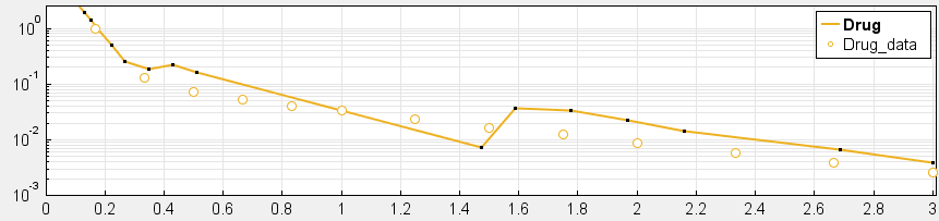
_ Tolerances are too low to simulate at the order of magnitude of the data. Absolute Tolerance: 0.001, Relative Tolerance: 0.01_

_ Sufficiently high tolerances. Absolute Tolerance: 1e-8, Relative Tolerance: 1e-5_

5. Have you checked the tolerances and stopping criteria of your optimization algorithm? The goal for your optimization should be that it terminates because it meets the imposed tolerances rather than because it exceeds the maximum number of iterations. Optimization algorithms terminate the estimation based on tolerances and stopping criteria. An example of a tolerance here is that you specify the precision with which you want to estimate a certain parameter, e.g. Cl with a precision down to 0.1 ml/hour. If these tolerances and stopping criteria are not set properly, your optimization could terminate early (leading to loss of precision in the estimation) or late (leading to unnecessarily long optimization compute times).

6. Have you considered structural and practical identifiability of your parameters? In your model, there might exist values for two (or more) parameters that result in a very similar model response. When estimating these parameters, the objective function will be very similar for these two parameters, resulting in the optimization algorithm not being able to find a unique set of parameter estimates. This effect is sometimes called aliasing and is a structural identifiability problem. An example would be if you have parallel enzymatic (Km, Vm) and linear clearance (Cl) routes. Practical identifiability occurs when there is not enough data available to sufficiently constrain the parameters you are estimating. An example is estimating the intercompartmental clearance (Q12), when you only have data on the central compartment of a two-compartment model. Another example would be that your data does not capture the process you are trying to estimate, e.g. you don’t have data on the absorption phase but are trying to estimate the absorption constant (Ka).

7. Have you considered trying another optimization algorithm? SimBiology supports a range of optimization algorithms, depending on the toolboxes you have installed. There is no single answer as to which algorithm you should use but some general guidelines can help in selecting the best algorithm.

• Non-linear regression: If your aim is to estimate parameters estimates for each group in your dataset (unpooled) or for all groups (pooled), you can use non-linear regression estimation methods. The optimization algorithms can be broken down into local and global optimization algorithms. You can use a local optimization algorithm when you have good initial estimates for the parameters you are trying to estimate. Each of the local optimization functions has a different default optimization algorithm: fminsearch (Nelder-Mead/downhill simplex search method), fmincon (interior-point), fminunc (quasi-newton), nlinfit (Levenberg-Marquardt), lsqcurvefit, lsqnonlin (both trust-region-reflective algorithm). As a default, we would recommend using lsqnonlin if you have access to the Optimization Toolbox. Note that all but the fminsearch algorithm are gradient based. If a gradient based algorithm fails to find suitable estimates, you can try fminsearch and see whether that improves the optimization. All local optimization algorithms can get “stuck” in a local minimum of the objective function and might therefore fail to reach the true minimum. Global optimization algorithms are developed to find the absolute minimum of the objective function. You can use global optimization algorithms when your fitting task results in different parameter estimates when repeated with different initial values (in other words, your optimization is getting stuck in local minima). You are more likely to encounter this as you increase the number of parameters you are estimating, as you increase the parameter space you are exploring (in other words, the bounds you are imposing on your estimates) and when you have poor initial estimates (in other words, your initial estimates are potentially very far from the estimates that correspond with the minimum of the objective function). A disadvantage of global optimization algorithms is that these algorithms are much more computationally expensive – they often take significantly more time to converge than the local optimization methods do. When using global optimization methods, we recommend using SimBiology’s built-in scattersearch algorithm, combined with lsqnonlin as a local solver. If you have access to the Global Optimization Toolbox, you can try the functions ga (genetic algorithm), patternsearch and particleswarm. Note that some of the global optimization algorithms, including scattersearch, lend themselves well to be accelerated using parallel or distributed computing.

• Estimate category-specific parameters: If you want to estimate category-specific parameters for multiple subjects, e.g. you have 10 male and 10 female subjects in your dataset and you want to estimate a separate clearance value for each gender while all other parameters will be gender-independent, you can also use non-linear regression. Please refer to this example in the documentation.

• Non-linear mixed effects: If your data represents a population of individuals where you think there could be significant inter-individual variability you can use mixed effects modeling to estimate the fixed and random effects present in your population, while also understanding covariance between different parameters you are trying to estimate. When performing mixed effects estimation, it is advisable to perform fixed effects estimation in order to obtain reasonable initial estimates for the mixed effects estimation. SimBiology supports two estimation functions: nlmefit (LME, RELME, FO or FOCE algorithms), and nlmefitsa (Stochastic Approximation Expectation-Maximization). Sometimes, these solvers might seem to struggle to converge. In that case, it is worthwhile determining whether your (objective) function tolerance is set too low and increasing the tolerance somewhat.

8. Does your optimization get stuck? Sometimes, the optimization algorithm can get stuck at a certain iteration. For a particular iteration, the parameter values that model is simulated with as part of the optimization process, can cause the model to be in a state where the ODE solver needs to take very small time-steps to achieve the tolerances (e.g. very rapid changes of model responses). Solutions can include: changing your initial estimates, imposing lower and upper bounds on the parameters you are trying to estimate, selecting to a different solver, easing solver tolerances (only where possible, see also “Visually inspect data and model response”).

9. Are you using the proportional error model? The objective function for the proportional error model contains a term where your response data is part of the denominator. As response variables get close to zero or are exactly zero, this effectively means the objective function contains one or more terms that divide by zero, causing errors or at least very slow iterations of your optimization algorithm. You can try to change the error model to constant or combined to circumvent this problem. Alternatively, you can define separate error models for each response: proportional for those responses that don’t have measurements that contain values close to zero and a constant error model for those responses that do.

Dear all,

I am new to SimBiology. I am doing my research in Molecular Communication. Recently I have found out that SimBiology can be used for simulating the Bit Error Rate performance of molecular Communication systems. Please help me to find good reference materials/examples for using SimBiology as a simulation tool for Molecular Communications.

Thank you.

Tomorrow (Wednesday, January 23) during Rosa's Impact of Modeling & Simulation in Drug Development webinar series, Chi-Chung Li, a Senior Scientist at Genentech, will present a case study where SimBiology was used to create a QSP model that enhanced decision making in a Phase I trial.

Sign up now and have the ability to ask questions at the end of the webinar, or access the archived version later: https://www.rosaandco.com/webinars/2019/phase-i-clinical-decision-making-qsp-case-study

AI and ACoP, hype or real?