주요 콘텐츠

다음에 대한 결과:

Function Syntax Design Conundrum
As a MATLAB enthusiast, I particularly enjoy Steve Eddins' blog and the cool things he explores. MATLAB's new argument blocks are great, but there's one frustrating limitation that Steve outlined beautifully in his blog post "Function Syntax Design Conundrum": cases where an argument should accept both enumerated values AND other data types.
Steve points out this could be done using the input parser, but I prefer having tab completions and I'm not a fan of maintaining function signature JSON files for all my functions.
Personal Context on Enumerations
To be clear: I honestly don't like enumerations in any way, shape, or form. One reason is how awkward they are. I've long suspected they're simply predefined constructor calls with a set argument, and I think that's all but confirmed here. This explains why I've had to fight the enumeration system when trying to take arguments of many types and normalize them to enumerated members, or have numeric values displayed as enumerated members without being recast to the superclass every operation.
The Discovery
While playing around extensively with metadata for another project, I realized (and I'm entirely unsure why it took so long) that the properties of a metaclass object are just, in many cases, the attributes of the classdef. In this realization, I found a solution to Steve's and my problem.
To be clear: I'm not in love with this solution. I would much prefer a better approach for allowing variable sets of membership validation for arguments. But as it stands, we don't have that, so here's an interesting, if incredibly hacky, solution.
If you call struct() on a metaclass object to view its hidden properties, you'll notice that in addition to the public "Enumeration" property, there's a hidden "Enumerable" property. They're both logicals, which implies they're likely functionally distinct. I was curious about that distinction and hoped to find some functionality by intentionally manipulating these values - and I did, solving the exact problem Steve mentions.
The Problem Statement
We have a function with an argument that should allow "dual" input types: enumerated values (Steve's example uses days of the week, mine uses the "all" option available in various dimension-operating functions) AND integers. We want tab completion for the enumerated values while still accepting the numeric inputs.
A Solution for Tab-Completion Supported Arguments
Rather than spoil Steve's blog post, let me use my own example: implementing a none() function. The definition is simple enough tf = ~any(A, dim); but when we wrap this in another function, we lose the tab-completion that any() provides for the dim argument (which gives you "all"). There's no great way to implement this as a function author currently - at least, that's well documented.
So here's my solution:
%% Example Function Implementation
% This is a simple implementation of the DimensionArgument class for implementing dual type inputs that allow enumerated tab-completion.
function tf = none(A, dim)
arguments(Input)
A logical;
dim DimensionArgument = DimensionArgument(A, true);
end
% Simple example (notice the use of uplus to unwrap the hidden property)
tf = ~any(A, +dim);
end
I like this approach because the additional work required to implement it, once the enumeration class is initialized, is minimal. Here are examples of function calls, note that the behavior parallels that of the MATLAB native-style tab-completion:
%% Test Data
% Simple logical array for testing
A = randi([0, 1], [3, 5], "logical");
%% Example function calls
tf = none(A, "all"); % This is the tab-completion it's 1:1 with MATLABs behavior
tf = none(A, [1, 2]); % We can still use valid arguments (validated in the constructor)
tf = none(A); % Showcase of the constructors use as a default argument generator
How It Works
What makes this work is the previously mentioned Enumeration attribute. By setting Enumeration = false while still declaring an enumeration block in the classdef file, we get the suggested members as auto-complete suggestions. As I hinted at, the value of enumerations (if you don't subclass a builtin and define values with the someMember (1) syntax) are simply arguments to constructor calls.
We also get full control over the storage and handling of the class, which means we lose the implicit storage that enumerations normally provide and are responsible for doing so ourselves - but I much prefer this. We can implement internal validation logic to ensure values that aren't in the enumerated set still comply with our constraints, and store the input (whether the enumerated member or alternative type) in an internal property.
As seen in the example class below, this maintains a convenient interface for both the function caller and author the only particuarly verbose portion is the conversion methods... Which if your willing to double down on the uplus unwrapping context can be avoided. What I have personally done is overload the uplus function to return the input (or perform the identity property) this allowss for the uplus to be used universally to unwrap inputs and for those that cant, and dont have a uplus definition, the value itself is just returned:
classdef(Enumeration = false) DimensionArgument % < matlab.mixin.internal.MatrixDisplay
%DimensionArgument Enumeration class to provide auto-complete on functions needing the dimension type seen in all()
% Enumerations are just macros to make constructor calls with a known set of arguments. Declaring the 'all'
% enumeration member means this class can be set as the type for an input and the auto-completion for the given
% argument will show the enumeration members, allowing tab-completion. Declaring the Enumeration attribute of
% the class as false gives us control over the constructor and internal implementation. As such we can use it
% to validate the numeric inputs, in the event the 'all' option was not used, and return an object that will
% then work in place of valid dimension argument options.
%% Enumeration members
% These are the auto-complete options you'd like to make available for the function signature for a given
% argument.
enumeration(Description="Enumerated value for the dimension argument.")
all
end
%% Properties
% The internal property allows the constructor's input to be stored; this ensures that the value is store and
% that the output of the constructor has the class type so that the validation passes.
% (Constructors must return the an object of the class they're a constructor for)
properties(Hidden, Description="Storage of the constructor input for later use.")
Data = [];
end
%% Constructor method
% By the magic of declaring (Enumeration = false) in our class def arguments we get full control over the
% constructor implementation.
%
% The second argument in this specific instance is to enable the argument's default value to be set in the
% arguments block itself as opposed to doing so in the function body... I like this better but if you didn't
% you could just as easily keep the constructor simple.
methods
function obj = DimensionArgument(A, Adim)
%DimensionArgument Initialize the dimension argument.
arguments
% This will be the enumeration member name from auto-completed entries, or the raw user input if not
% used.
A = [];
% A flag that indicates to create the value using different logic, in this case the first non-singleton
% dimension, because this matches the behavior of functions like, all(), sum() prod(), etc.
Adim (1, 1) logical = false;
end
if(Adim)
% Allows default initialization from an input to match the aforemention function's behavior
obj.Data = firstNonscalarDim(A);
else
% As a convenience for this style of implementation we can validate the input to ensure that since we're
% suppose to be an enumeration, the input is valid
DimensionArgument.mustBeValidMember(A);
% Store the input in a hidden property since declaring ~Enumeration means we are responsible for storing
% it.
obj.Data = A;
end
end
end
%% Conversion methods
% Applies conversion to the data property so that implicit casting of functions works. Unfortunately most of
% the MathWorks defined functions use a different system than that employed by the arguments block, which
% defers to the class defined converter methods... Which is why uplus (+obj) has been defined to unwrap the
% data for ease of use.
methods
function obj = uplus(obj)
obj = obj.Data;
end
function str = char(obj)
str = char(obj.Data);
end
function str = cellstr(obj)
str = cellstr(obj.Data);
end
function str = string(obj)
str = string(obj.Data);
end
function A = double(obj)
A = double(obj.Data);
end
function A = int8(obj)
A = int8(obj.Data);
end
function A = int16(obj)
A = int16(obj.Data);
end
function A = int32(obj)
A = int32(obj.Data);
end
function A = int64(obj)
A = int64(obj.Data);
end
end
%% Validation methods
% These utility methods are for input validation
methods(Static, Access = private)
function tf = isValidMember(obj)
%isValidMember Checks that the input is a valid dimension argument.
tf = (istext(obj) && all(obj == "all", "all")) || (isnumeric(obj) && all(isint(obj) & obj > 0, "all"));
end
function mustBeValidMember(obj)
%mustBeValidMember Validates that the input is a valid dimension argument for the dim/dimVec arguments.
if(~DimensionArgument.isValidMember(obj))
exception("JB:DimensionArgument:InvalidInput", "Input must be an integer value or the term 'all'.")
end
end
end
%% Convenient data display passthrough
methods
function disp(obj, name)
arguments
obj DimensionArgument
name string {mustBeScalarOrEmpty} = [];
end
% Dispatch internal data's display implementation
display(obj.Data, char(name));
end
end
end
In the event you'd actually play with theres here are the function definitions for some of the utility functions I used in them, including my exception would be a pain so i wont, these cases wont use it any...
% Far from my definition isint() but is consistent with mustBeInteger() for real numbers but will suffice for the example
function tf = isint(A)
arguments
A {mustBeNumeric(A)};
end
tf = floor(A) == A
end
% Sort of the same but its fine
function dim = firstNonscalarDim(A)
arguments
A
end
dim = [find(size(A) > 1, 1), 0];
dim(1) = dim(1);
end
This week's Graphics and App Building blog article guides chart authors and app builders through the process of designing for a specific theme or creating theme-responsive charts and apps.
  • Learn how dark theme may impacts charts and apps
  • Discover best practices for theme-adaptive workflows
  • Step-by-step examples for both script-based plots and advanced custom charts and UI components
  • Discover new tools like ThemeChangedFcn, getTheme, and fliplightness
I am thrilled python interoperability now seems to work for me with my APPLE M1 MacBookPro and MATLAB V2025a. The available instructions are still, shall we say, cryptic. Here is a summary of my interaction with GPT 4o to get this to work.
===========================================================
MATLAB R2025a + Python (Astropy) Integration on Apple Silicon (M1/M2/M3 Macs)
===========================================================
Author: D. Carlsmith, documented with ChatGPT
Last updated: July 2025
This guide provides full instructions, gotchas, and workarounds to run Python 3.10 with MATLAB R2025a (Apple Silicon/macOS) using native ARM64 Python and calling modules like Astropy, Numpy, etc. from within MATLAB.
===========================================================
Overview
===========================================================
- MATLAB R2025a on Apple Silicon (M1/M2/M3) runs as "maca64" (native ARM64).
- To call Python from MATLAB, the Python interpreter must match that architecture (ARM64).
- Using Intel Python (x86_64) with native MATLAB WILL NOT WORK.
- The cleanest solution: use Miniforge3 (Conda-forge's lightweight ARM64 distribution).
===========================================================
1. Install Miniforge3 (ARM64-native Conda)
===========================================================
In Terminal, run:
curl -LO https://github.com/conda-forge/miniforge/releases/latest/download/Miniforge3-MacOSX-arm64.sh
bash Miniforge3-MacOSX-arm64.sh
Follow prompts:
- Press ENTER to scroll through license.
- Type "yes" when asked to accept the license.
- Press ENTER to accept the default install location: ~/miniforge3
- When asked:
Do you wish to update your shell profile to automatically initialize conda? [yes|no]
Type: yes
===========================================================
2. Restart Terminal and Create a Python Environment for MATLAB
===========================================================
Run the following:
conda create -n matlab python=3.10 astropy numpy -y
conda activate matlab
Verify the Python path:
which python
Expected output:
/Users/YOURNAME/miniforge3/envs/matlab/bin/python
===========================================================
3. Verify Python + Astropy From Terminal
===========================================================
Run:
python -c "import astropy; print(astropy.__version__)"
Expected output:
6.x.x (or similar)
===========================================================
4. Configure MATLAB to Use This Python
===========================================================
In MATLAB R2025a (Apple Silicon):
clear classes
pyenv('Version', '/Users/YOURNAME/miniforge3/envs/matlab/bin/python')
py.sys.version
You should see the Python version printed (e.g. 3.10.18). No error means it's working.
===========================================================
5. Gotchas and Their Solutions
===========================================================
❌ Error: Python API functions are not available
→ Cause: Wrong architecture or broken .dylib
→ Fix: Use Miniforge ARM64 Python. DO NOT use Intel Anaconda.
❌ Error: Invalid text character (↑ points at __version__)
→ Cause: MATLAB can’t parse double underscores typed or pasted
→ Fix: Use: py.getattr(module, '__version__')
❌ Error: Unrecognized method 'separation' or 'sec'
→ Cause: MATLAB can't reflect dynamic Python methods
→ Fix: Use: py.getattr(obj, 'method')(args)
===========================================================
6. Run Full Verification in MATLAB
===========================================================
Paste this into MATLAB:
% Set environment
clear classes
pyenv('Version', '/Users/YOURNAME/miniforge3/envs/matlab/bin/python');
% Import modules
coords = py.importlib.import_module('astropy.coordinates');
time_mod = py.importlib.import_module('astropy.time');
table_mod = py.importlib.import_module('astropy.table');
% Astropy version
ver = char(py.getattr(py.importlib.import_module('astropy'), '__version__'));
disp(['Astropy version: ', ver]);
% SkyCoord angular separation
c1 = coords.SkyCoord('10h21m00s', '+41d12m00s', pyargs('frame', 'icrs'));
c2 = coords.SkyCoord('10h22m00s', '+41d15m00s', pyargs('frame', 'icrs'));
sep_fn = py.getattr(c1, 'separation');
sep = sep_fn(c2);
arcsec = double(sep.to('arcsec').value);
fprintf('Angular separation = %.3f arcsec\n', arcsec);
% Time difference in seconds
Time = time_mod.Time;
t1 = Time('2025-01-01T00:00:00', pyargs('format','isot','scale','utc'));
t2 = Time('2025-01-02T00:00:00', pyargs('format','isot','scale','utc'));
dt = py.getattr(t2, '__sub__')(t1);
seconds = double(py.getattr(dt, 'sec'));
fprintf('Time difference = %.0f seconds\n', seconds);
% Astropy table display
tbl = table_mod.Table(pyargs('names', {'a','b'}, 'dtype', {'int','float'}));
tbl.add_row({1, 2.5});
tbl.add_row({2, 3.7});
disp(tbl);
===========================================================
7. Optional: Automatically Configure Python in startup.m
===========================================================
To avoid calling pyenv() every time, edit your MATLAB startup:
edit startup.m
Add:
try
pyenv('Version', '/Users/YOURNAME/miniforge3/envs/matlab/bin/python');
catch
warning("Python already loaded.");
end
===========================================================
8. Final Notes
===========================================================
- This setup avoids all architecture mismatches.
- It uses a clean, minimal ARM64 Python that integrates seamlessly with MATLAB.
- Do not mix Anaconda (Intel) with Apple Silicon MATLAB.
- Use py.getattr for any Python attribute containing underscores or that MATLAB can't resolve.
You can now run NumPy, Astropy, Pandas, Astroquery, Matplotlib, and more directly from MATLAB.
===========================================================
Hi everyone,
Please check out our new book "Generative AI for Trading and Asset Management".
GenAI is usually associated with large language models (LLMs) like ChatGPT, or with image generation tools like MidJourney, essentially, machines that can learn from text or images and generate text or images. But in reality, these models can learn from many different types of data. In particular, they can learn from time series of asset returns, which is perhaps the most relevant for asset managers.
In our book (amazon.com link), we explore both the practical applications and the fundamental principles of GenAI, with a special focus on how these technologies apply to trading and asset management.
The book is divided into two broad parts:
Part 1 is written by Ernie Chan, noted author of Quantitative Trading, Algorithmic Trading, and Machine Trading. It starts with no-code applications of GenAI for traders and asset managers with little or no coding experience. After that, it takes readers on a whirlwind tour of machine learning techniques commonly used in finance.
Part 2, written by Hamlet, covers the fundamentals and technical details of GenAI, from modeling to efficient inference. This part is for those who want to understand the inner workings of these models and how to adapt them to their own custom data and applications. It’s for anyone who wants to go beyond the high-level use cases, get their hands dirty, and apply, and eventually improve these models in real-world practical applications.
Readers can start with whichever part they want to explore and learn from.
The Graphics and App Building Blog just launched its first article on R2025a features, authored by Chris Portal, the director of engineering for the MATLAB graphics and app building teams.
Over the next few months, we'll publish a series of articles that showcase our updated graphics system, introduce new tools and features, and provide valuable references enriched by the perspectives of those involved in their development.
To stay updated, you can subscribe to the blog (look for the option in the upper left corner of the blog page). We also encourage you to join the conversation—your comments and questions under each article help shape the discussion and guide future content.
What is a rough number? What can they be used for? Today I'll take you down a journey into the land of prime numbers (in MATLAB). But remember that a journey is not always about your destination, but about what you learn along the way. And so, while this will be all about primes, and specifically large primes, before we get there we need some background. That will start with rough numbers.
Rough numbers are what I would describe as wannabe primes. Almost primes, and even sometimes prime, but often not prime. They could've been prime, but may not quite make it to the top. (If you are thinking of Marlon Brando here, telling us he "could've been a contender", you are on the right track.)
Mathematically, we could call a number k-rough if it is evenly divisible by no prime smaller than k. (Some authors will use the term k-rough to denote a number where the smallest prime factor is GREATER than k. The difference here is a minor one, and inconsequential for my purposes.) And there are also smooth numbers, numerical antagonists to the rough ones, those numbers with only small prime factors. They are not relevant to the topic today, even though smooth numbers are terribly valuable tools in mathematics. Please forward my apologies to the smooth numbers.
Have you seen rough numbers in use before? Probably so, at least if you ever learned about the sieve of Eratosthenes for prime numbers, though probably the concept of roughness was never explicitly discussed at the time. The sieve is simple. Suppose you wanted a list of all primes less than 100? (Without using the primes function itself.)
% simple sieve of Eratosthenes
Nmax = 100;
N = true(1,Nmax); % A boolean vector which when done, will indicate primes
N(1) = false; % 1 is not a prime by definition
nextP = find(N,1,'first'); % the first prime is 2
while nextP <= sqrt(Nmax)
% flag multiples of nextP as not prime
N(nextP*nextP:nextP:end) = false;
% find the first element after nextP that remains true
nextP = nextP + find(N(nextP+1:end),1,'first');
end
primeList = find(N)
primeList = 1×25
2 3 5 7 11 13 17 19 23 29 31 37 41 43 47 53 59 61 67 71 73 79 83 89 97
<mw-icon class=""></mw-icon>
Indeed, that is the set of all 25 primes not exceeding 100. If you think about how the sieve worked, it first found 2 is prime. Then it discarded all integer multiples of 2. The first element after 2 that remains as true is 3. 3 is of course the second prime. At each pass through the loop, the true elements that remain correspond to numbers which are becoming more and more rough. By the time we have eliminated all multiples of 2, 3, 5, and finally 7, everything else that remains below 100 must be prime! The next prime on the list we would find is 11, but we have already removed all multiples of 11 that do not exceed 100, since 11^2=121. For example, 77 is 11*7, but we already removed it, because 77 is a multiple of 7.
Such a simple sieve to find primes is great for small primes. However is not remotely useful in terms of finding primes with many thousands or even millions of decimal digits. And that is where I want to go, eventually. So how might we use roughness in a useful way? You can think of roughness as a way to increase the relative density of primes. That is, all primes are rough numbers. In fact, they are maximally rough. But not all rough numbers are primes. We might think of roughness as a necessary, but not sufficient condition to be prime.
How many primes lie in the interval [1e6,2e6]?
numel(primes(2e6)) - numel(primes(1e6))
ans = 70435
There are 70435 primes greater than 1e6, but less than 2e6. Given there are 1 million natural numbers in that set, roughly 7% of those numbers were prime. Next, how many 100-rough numbers lie in that same interval?
N = (1e6:2e6)';
roughInd = all(mod(N,primes(100)) > 0,2);
sum(roughInd)
ans = 120571
That is, there are 120571 100-rough numbers in that interval, but all those 70435 primes form a subset of the 100-rough numbers. What does this tell us? Of the 1 million numbers in that interval, approximately 12% of them were 100-rough, but 58% of the rough set were prime.
The point being, if we can efficiently identify a number as being rough, then we can substantially increase the chance it is also prime. Roughness in this sense is a prime densifier. (Is that even a word? It is now.) If we can reduce the number of times we need to perform an explicit isprime test, that will gain greatly because a direct test for primality is often quite costly in CPU time, at least on really large numbers.
In my next post, I'll show some ways we can employ rough numbers to look for some large primes.
Overview
Authors:
  • Narayanaswamy P.R. Iyer
  • Provides Simulink models for various PWM techniques used for inverters
  • Presents vector and direct torque control of inverter-fed AC drives and fuzzy logic control of converter-fed AC drives
  • Includes examples, case studies, source codes of models, and model projects from all the chapters.
About this book
Successful development of power electronic converters and converter-fed electric drives involves system modeling, analyzing the output voltage, current, electromagnetic torque, and machine speed, and making necessary design changes before hardware implementation. Inverters and AC Drives: Control, Modeling, and Simulation Using Simulink offers readers Simulink models for single, multi-triangle carrier, selective harmonic elimination, and space vector PWM techniques for three-phase two-level, multi-level (including modular multi-level), Z-source, Quasi Z-source, switched inductor, switched capacitor and diode assisted extended boost inverters, six-step inverter-fed permanent magnet synchronous motor (PMSM), brushless DC motor (BLDCM) and induction motor (IM) drives, vector-controlled PMSM, IM drives, direct torque-controlled inverter-fed IM drives, and fuzzy logic controlled converter-fed AC drives with several examples and case studies. Appendices in the book include source codes for all relevant models, model projects, and answers to selected model projects from all chapters. 
This textbook will be a valuable resource for upper-level undergraduate and graduate students in electrical and electronics engineering, power electronics, and AC drives. It is also a hands-on reference for practicing engineers and researchers in these areas.
  
Sonesson
Sonesson
최근 활동: 2024년 11월 5일

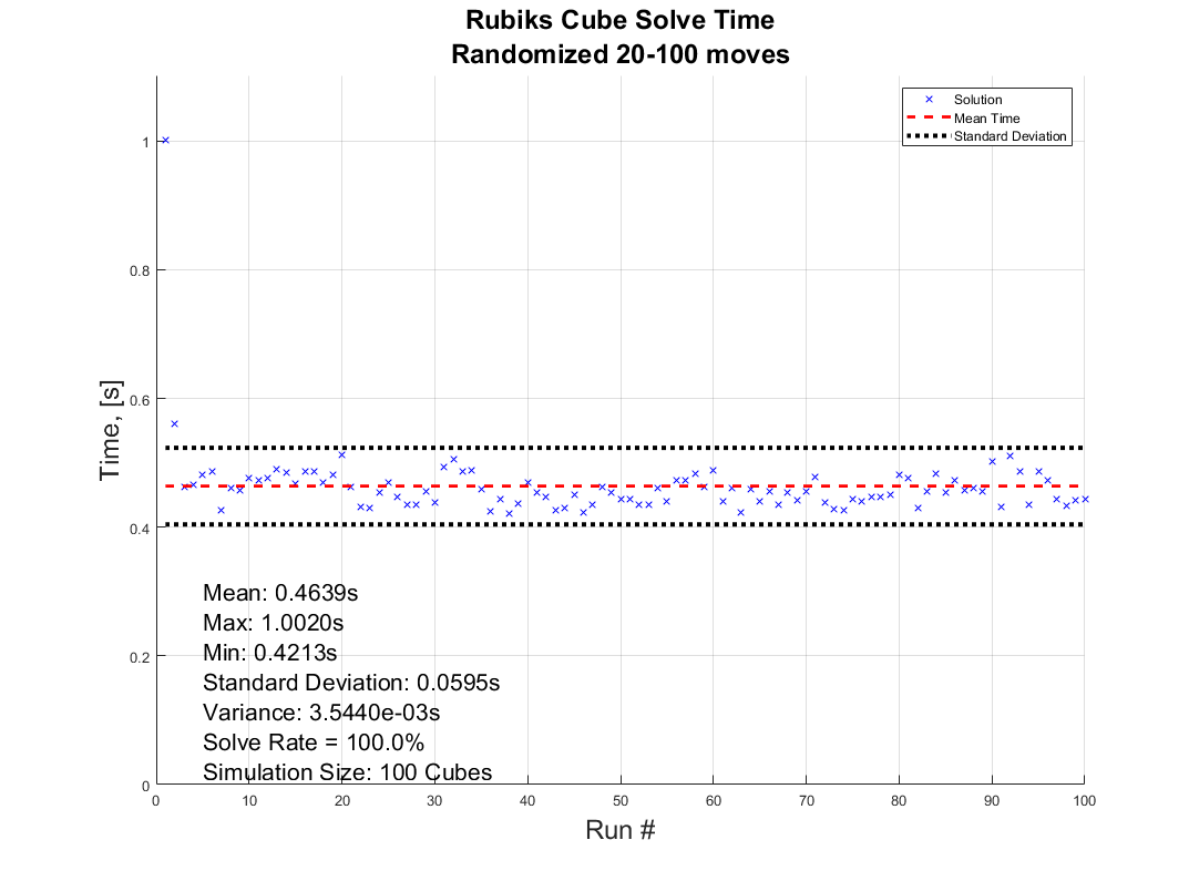
About a year ago, I made a rubix cube solver with the goal of solving a cube faster than I could in real life. It was a fun and educating project, and while it is a long way from optimal, I finished with satisfying results.
How the solver is made is a story for another time, but I always wanted to have a 3D illustration of how the moves are performed to reach the solved state. Lacking the motivation at the time, the illustrative part was forgotten... Untill a couple of weeks ago when I found out about the MATLAB Shorts Mini Hack. It was the perfect motivation to finish up!
This post will detail my entry and remixes (you should check them out before reading!) in this years mini hack. I am not a man to spare any detail, and I've recently saved up a bunch of characters from being limited to 2000, so it may be a bit wordy, but I'll try to keep it entertaining. How it works, lessons learned, sidetracks, pitfalls found, and everything in between is detailed here. So feel free to peruse the sections and pick the ones that sound interesting!
How can I make it move?
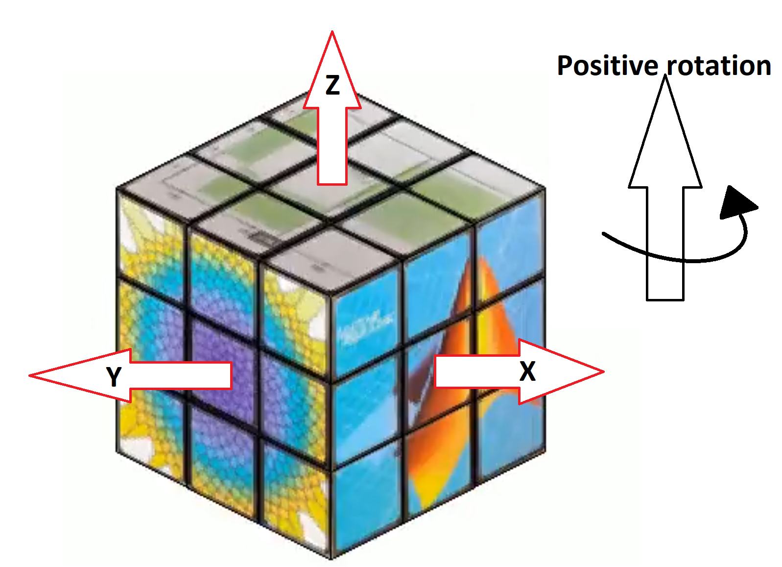
Intuativly one would use standard rubix notation to determine the moves, but due to the character limitation and me wanting the ability to rotate the middle rows and the cube as a whole I decided against this.
At the tippy top, there is an 3xn character array, MS, containing the movement sequence of the cube. The three rows contains:
  1. The axis to rotate around. - Defined by character x, y, z, or p (none of them).
  2. The row to rotate. - Defined by character 1, 2, 3, or 4 (all of them)
  3. The direction of the rotation. - Defined by character n, or p (negative or positive)
The rows are ordered from largest to smallest coordinate value along the axis of rotation. If a pause is selected, the program does not really care which character is chosen for the row and direction.
"But how many moves can I make within the time?" As many, or few, as you want.
Well... As long as you want 96 or less moves that is. The function alters the angular speed of the rotations to fit them all within the 96 frame window. But since we iterate through the cube (more on that later) we need to ensure that a move has completely finished before starting another move, or the cube will start looking like a contortionist.
If there is remaining time before the 96 frames are up (due to the timing of the angular speed), the cube politely pauses and waits for the last coule of frames to pass.
The hardest part is finding a sequence short enough to not look like the cube is flailing wildly during its 4 seconds of fame, but long enough to make some interesting pattern like the tetris shuffle in my original entry! Preferably while still being a perfect loop.
I would go on about good seamless loop mechanics, but Vasilis Bellos already made the great post "Creating seamless loop animations by zooming in" last week so I'll just sum it up to make sure to end right before the place you start.
Easy, right? Now go make your own!
Tip: Use the camera rotation to your advantage! Wanting to showcase all sides of the Mathworks cube for as long as possible, I needed a short movement sequence which gives lower angular speed. I cut out two moves from the sequence by making the camera rotate 180 degrees to finish my perfect loop at a different set of coordinates from where I started!
How did you make the cube so beautiful (MathWorks motive)?
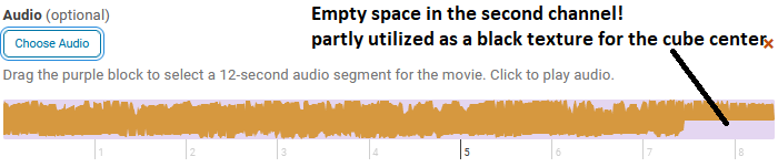
A lot of credit should go to Tomoaki Takagi and his entry. I am a sucker for utilizing things for purposes they were not intended to be used for, and he did just that.
We are not allowed to upload images or data in the contest. But we are allowed to optionally upload some background audio for the video. The key is to realise that this audio is stored in the same place as the contest entry. Meaning we can access the "audio.wav" file we just uploaded to the contest.
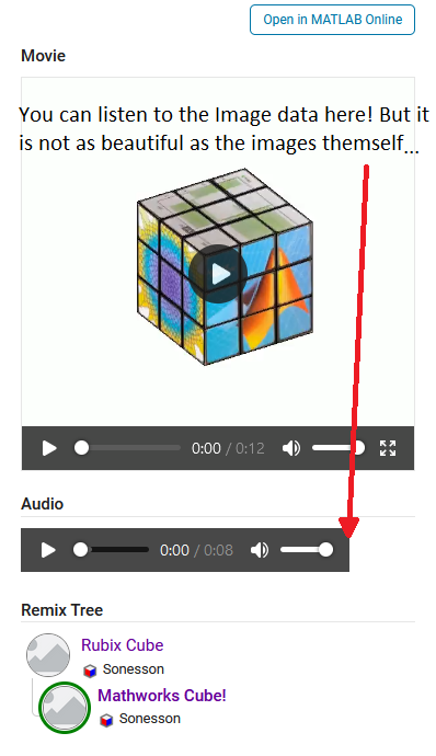
An audio file is really just a long row of values between -1 and 1. So... if one were to take a picture of every side of a MathWorks cube laying around on the desk, splice the images into 54 seperate textures, scale the intensities between 0 and 1, reshape them to a row, and save it as an .wav file using the audiowrite() function... One would have a bit too much free time, but also a terrible sounding audio file with image data encoded.
There is one small problem however. As you might have noticed, the audio of most entries sound... rough. This is because of an file compression (or something of the like) applied to files over a certain length when you upload them to the contest. This also applies to audio files filled with image data that does not take particularly well to getting squeezed.
The solution? Compress it yourself (carefully)! Again I looked at Tomoaki's entry, to see what length worked for him. His entry contained a 150x150x3 image upscaled by a factor 4. His image is not exactly sharp, and with 54 different textures needed for a cube, each side would be... about 3x3x3. While a bit poetic, we can not bring such dishonour to such a beautiful object! Luckily Tomoaki had not used the entire audio file for image storage. And he used mono sound (1 audio channel) for his entry and .wav files support stereo sound (2 aoudio channels) meaning I could utilize twice as much space netting me a neat, decent resolution of 28x28 pixels per face!
Don't forget to overwrite the audio on the last frame using audiowrite() however! Most people don't appreciate the sound of images. You should explore Tomoaki's entry for more information on this. The entry is short and easy to understand.
Summary: The audio file uploaded can be used to store image data instead of sound data. Just be careful about file length and size as compression won't treat you kindly!
How did you build the cube?
Excellent question, my dear watsson. Surfaces. Lots and lots of surfaces. This part is takes the most computation time. If anyone has some forbidden knowledge I don't know about here, feel free to correct and enlighten me!
We want to be able to assign each face of the cube a seperate texture, and to be able to move each face seperately without it morphing itself or other parts of the cube. Because of this, they can't be part of a meshgrid connecting each other. Instead we have to construct each surface individually. This takes a second, but is much better in my latest version (See more in the I crave speed section). Which in my earlier entries was a big deal because I was yet to learn about our lord and saviour, persistent variables through Timothy's beautiful entry: Refraction.
One could think a rubix cube has 54 faces, 9 on each side, but alas that is but an illusion. A rubix cube is infact 27 (26 if not counting the center) smaller cubes in a trench coat. Each with 6 sides. (As illustrated by William Dean's entry Is this cheating? posted while I'm writing this, thanks for the assist!).
Patch objects are all good and well when creating faces if you only want colors, which is the case in my first submission. But MATLAB surface objects are also 3D and have a property that allows them to be textured which we use in the later versions.
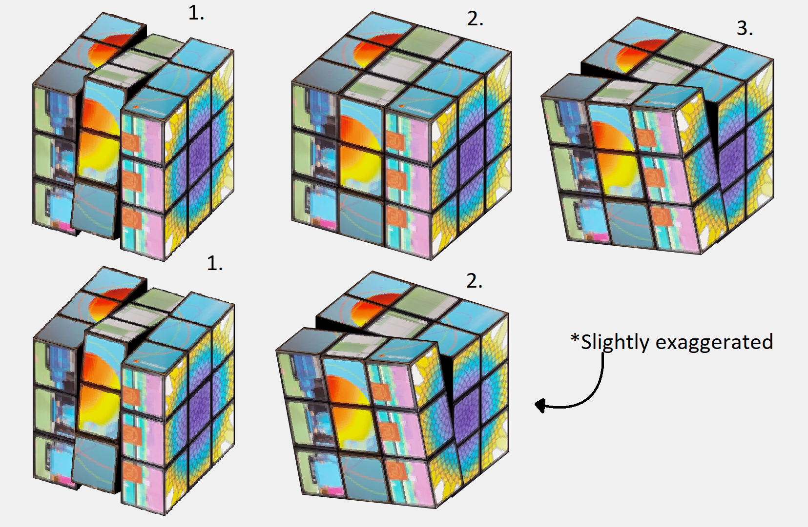
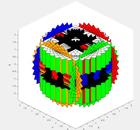
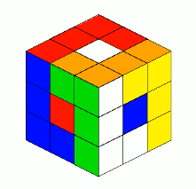
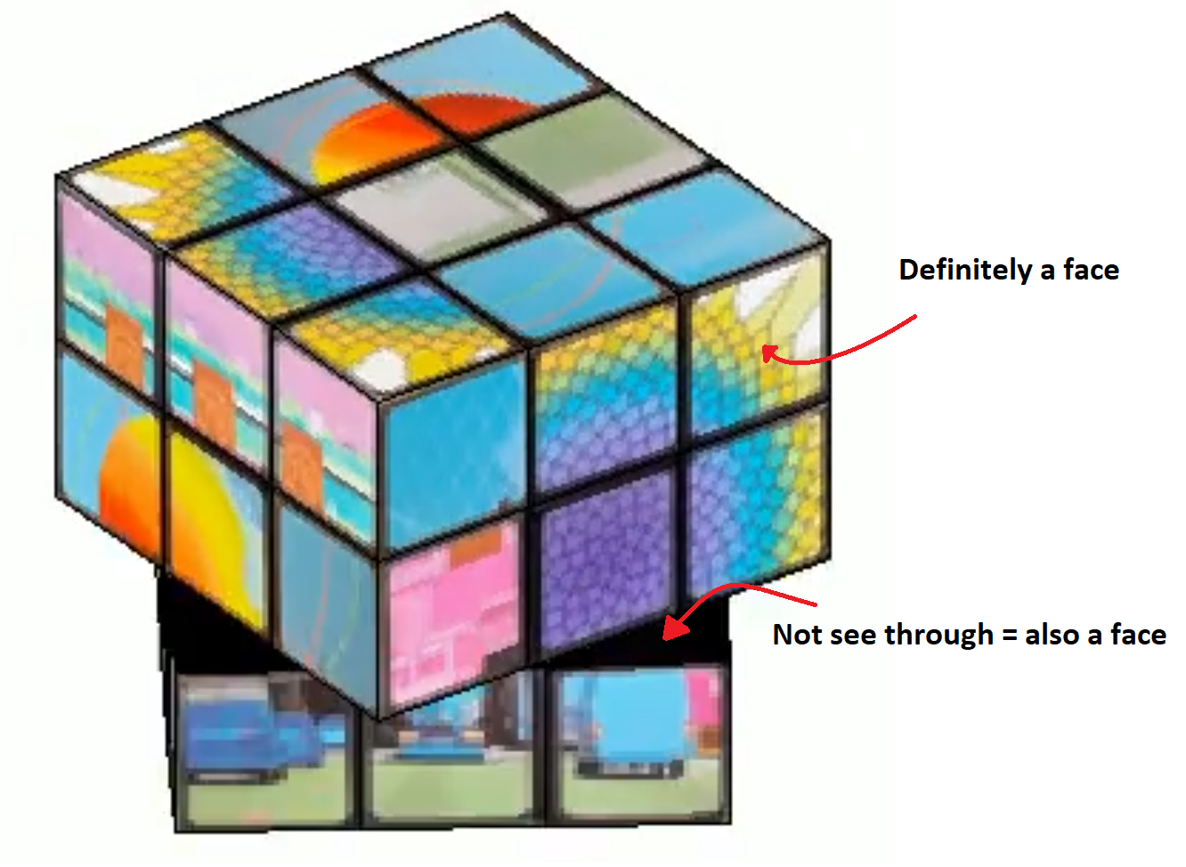
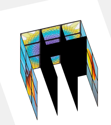
Thinking about the trench coat covered cubes, we can tell that on a physical cube we have 6 planes in each coordinate direction. 2 for each row of cubes. The faces pointing outward are textured and the faces pointing inward are typically black. That is how we will model our cube as well.
The above image shows how the cube looks during the process of building each face. You may think to yourself "Why do you only have 4 planes in a direction? Do we really need all 6 that you mentioned?" Yes. and if you could enhance and zoom the image like the movies, you would see a tiny gap between the "2" black central planes (this is a surprise tool that will help us later!). The 6 planes are necessary to cover up the cube's hollow interior from multiple viewing angles so we can not compromise it down to 4. Imagine flippnig the cube in the first image of this section and looking into the cube. If we had 4 planes, we would be able to see through the cube from one of the angles.
Summary: We imagine the cube as 3x3x3 smaller cubes. We build each side, inwards pointing or not. We make each face of these smaller cubes seperately using surface() to avoid morphing behavior and to allow the surfaces to be textured individually.
How does it move?
The trick is all about coordinates. Firstly, to make the cube move we need a couple of things:
  • Some indicator of how and what to move (a movement sequence, MS)
  • The speed at which it should move
  • A way to separate what verticies should and should not move
  • An operation to transform the coordinates of said verticies so they move
  • And of course we need to update the existing data and plot.
We are already familliar with the movement sequence from the first section, so I will spare you the repetition.
The speed of rotation is fairly simple, we have a number of moves defined in MS, and a number of frames to play with, 96. Simply find how many frames we can afford to allocate each move, and since each "rotation" of the cube is a quarter turn () we get . Pretty straight forward.
Now we need to know which verticies should and should not move. Here we use our surprise tool from the previous section! When building the cube, we add a slight offset separating the central planes. We can use this coordinate shift to separate the different planes from eachother. This would not be entierly possible if the central planes shared coordinates.
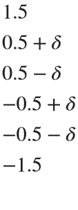
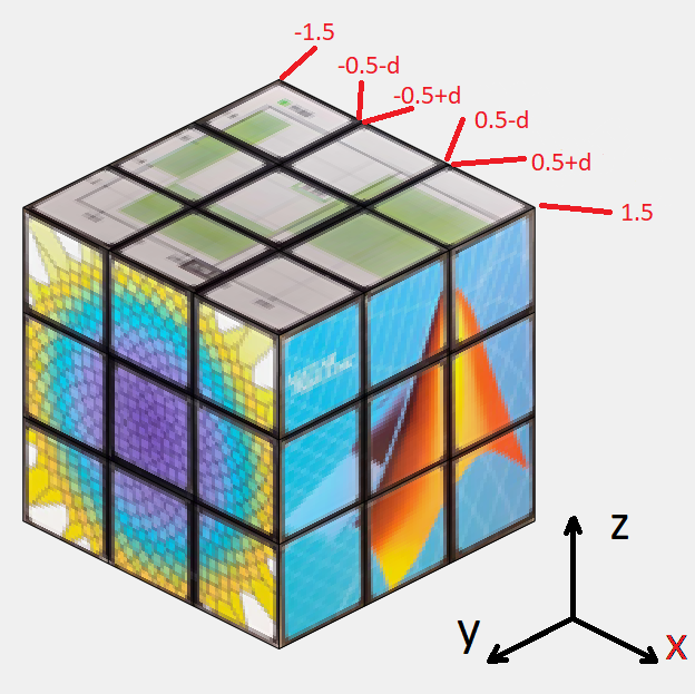
As an example, let's say the movement sequence dictates that we should rotate around x and we should choose the first row. Since the cube is centered around 0 and the planes have coordinates:
in all directions where δ is the small offset, we can easily seperate the first row by checking which faces have x coordinates higher than 0.5 in all 4 verticies. Simmilarly we check for 4 verticies in between ±0.5 for the 2nd row and values lower than -0.5 for the 3rd row. For rotating the entire cube, we can just select all faces. This works for all coordinate axis due to the symmetry that occurs when being centered around 0.
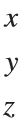
Now we need an operation to transform the coordinates of the verticies. We want to rotate some 3D coordinates around a specified coordinate axis. Sounds like the perfect job of a rotational matrix for me. This is why you stay in school kids.
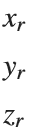
In case someone has never heard of a rotation matrix before, on the assumption that anyone using Matrix Laboratory is probably familliar with matrix math and basic linear algebra I'll keep this short. Basically, there are some standard matrices that will rotate a point [x,y,z] arount the origin of an axis. such that
=
Where the subscripts r denotes the rotated coordinates and ax the axis to rotate around.
These matricies are as follows:
Where θ is the angle with which you rotate the point. In our case the Angular speed.
Now, I define my own rotation matrices. This is because of one of three reasons:
  1. MATLAB does not have rotation function which rotates a point around a specified axis (this would baffle me)
  2. I am blind and could not see the correct function in the documentation (plausible)
  3. I am illiterate and can not read the documentation (improbable)
So we have everything we need! We just update the coordinate data of the affected surface objects, slap down a drawnow command for good measure, and call it an iteration!
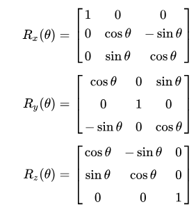
But I'd like to shine light on something that is both feature and flaw before we move on. 24 frames per second looks decent enough, but trained eyes can tell it is a bit choppy. Especially when things move fast. So we would like our movement as slow as possible. "Then why does the angular speed as defined above not always utilize all 96 frames to finish the movement sequence?" Because to a trained eye, what looks even more choppy is a rotation not finishing before another starts as the image shows below with a frame by frame on this effect.
By matching the angular speed to an integer number of frames (by using floor()) for each rotation, we will always complete the entire rotation before starting the next move.This is good because of the reason mentioned above (it looks better), but also because we will base the next rotation on the coordinates of the current position. So it also saves us having to do some extra math to get everything aligned and in position to select the correct faces every time we swap move.
Summary: We use a combination between clever choice of coordinates and some standard rotational matricies to shift the relevant verticies as dictated by the movement sequence by an angle. Being carefull to make each rotation precisely end on an integer number of frames so that the same method works next time.
I crave speed!
Well buckle up then bucko! Best part about programming is that the instant after you spend time making something, you learn something that trivialises it. Persistent variables were that for me this project. My 3rd remix is all about making it faster (in the works as we speak)! You know what they say; "Make it work, make it good, make it fast".
My biggest qualm about my earlier versions was the execution speeds. Every call of drawframe, I would have to rebuild all my surface object to make the cube and re-iterate all the movement of the cube up untill the current frame to ensure the rotations of all verticies, and thus faces, are correct.
Defining a variable as persistent allocates it's memory in a way that it is not removed between function calls. Perfect for being limited by 96 calls to the same function that does not accept iterative input.
Without persistent variables, we needed to remake the surfaces each call to drawframe. Worse still; since we dont know the positions of the surfaces in the previous frame, we also had to re-iterate all the movement of the cube. You may ask yourself "why could you not just calculate the surface position based on the frame, angular speed of rotation and previous moves?". While the position of each face is possible to anticipate effectively with a look up table (which would not fit in the character limit but could have been snuck in with the image data), the rotation of each face is a bit more complex to keep track of. Not an issue with plain colors, but a challange when using textured faces.
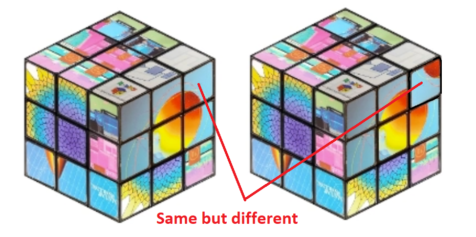
Using persistent variables as in my latest version solves theese two issues and makes the code run silky smooth compared to earlier. It now
  1. Removes the most time consuming part (creating surfaces) 95 out of 96 times, and
  2. Removes the need of re-iterating through all movement to catch up with all the rotations previously made.
It does however remove a neat function of the code; frame independency. The competition calls drawframe 96 times with the numbers 1:96, so frame independency it is not an issue as the previous frame is always the previous frame. However, if we now were to call the drawframe function with the values 1, 5 ,and 96, we would not recieve frame number 1, 5, and 96 of the animation as we would have before. Now there is an implicit need to call the function in with the frames in order.
An interesting thought that occured to me was; "If I can store the surface object in a variable, why could i not just copy it to another variable and edit it's properties instead of making a gazillion calls to surface()?" Well, turns out that is not possible because the surface object as stored in the workspace is really more of a pointer to the memory storing the object in the figure window rather than the value in the memory itself. If you copy surface_1 to surface_2 and change surface_2: you get the same change in surface_1.
Also, you might think;
"EWWW... I see nested for loops."
Yep. Is creating the coordinates for the surfaces vectorizable? Absolutely. Not even that hard either. Use combinations() with the possible x, y, and z coordinates and you got yourself the coordinates to every vertice of the cube. Use some fancy logic to determine which vertice goes where and vóila: all verticies neatly ordered ready to be made into surface objects. You could probably even use meshgrid() instead if that is more to your liking. The issue lies in the "made into surface objects" part. As stated, the repeated surface call is still needed to obtain seperate parts of memory to store the surface objects. You would still need as many loop iterations, though not nested. So I decided to leave the nested loops, as a treat, because it made it easier to determine the order and orientations of the textures when encoding them into the audio. After all, efficient coding is not only about the execution speed of the code, it is also about the writing speed of the coder. Or as textbook authors would say: "This is left as an excercise to the reader".
"Are all the inner planes necessary?"
Almost. We need 6 planes for the cube to not look hollow, but since the entire inside plane is black could we not just make it one big surface? No. Different part of the planes move with different rotations, and so can eventually end up as a part of another plane. To avoid morphing, they can not be connected. Also if the planes were solid, we would rotate into still standing planes when a row is angled (kind of like the black parts of the contorted cube earlier). However, we technically do not need the center of the 27 cubes in any scenario, and we could write some logic to not include those specific faces. This was not done for character limitation purposes. I figured that the slight tank in speed would be outweighed by the clean looks and the potential that you, the reader, could achieve when remixing this entry with those sweet sweet roughly 30 extra characters.
"Wait, are you looping... backwards?"
Yes! Looping backwards is a pretty neat trick. In this application it is mainly used to save characters, but runs in roughly the same time as a typical explicit preallocation would.
It works bacause we allocate the first loop value in the last variable element. It is the same principle as writing:
a(5) = 5
a = 1×5
0 0 0 0 5
<mw-icon class=""></mw-icon>
As you can see MATLAB will allocate memory for a 5 element vector despite us only specifying one element. So if we start from the back, MATLAB will do the front for us!
And here you can see how it holds up to not preallocating/typical allocation. Plus it gives the same result!
% No preallocation
tic
for i=1:1:10000
x(i) = i;
end
toc
Elapsed time is 0.012242 seconds.
% Typical Preallocation
tic
y=zeros(10000,1);
for i=1:1:10000
y(i) = i;
end
toc
Elapsed time is 0.005438 seconds.
% Backwards looping
tic
for i=10000:-1:1
z(i) = i;
end
toc
Elapsed time is 0.001842 seconds.
% And produces the same results!
all(z==x)
ans = logical
1
Summary: Persistent variables are really neat They keep their values between calls to functions. In terms of this contest they remove the need to re-iterate things, or for you to keep the state of the last frame without the need for rebuilding it every time.
Surface objects in the workspace are really just pointers to the surface objects in the figure window. This means that we unforttunately must call surface() for each face we want to create.
While initiating the surfaces, I use nested loops. Unnesting these loops is very doable with combination() and left as an excercise to the reader. You will still need the same total number of loop iterations to create all the surface objects, and the loops make texturing more convinient.
All 6 planes are necessary, but the central face of each "inside" plane is redundant and could be skipped at the cost of some additional logic.
Looping backwards is a cool trick to make MATLAB perform the preallocation of memory for you when iterating through a variable.
You get a cube, and you get a cube, and...
As earlier stated, in the "I crave speed!" section my 3 entries happen to follow the "Make it, make it good, make it fast" rule. But I did not just want to upload something that did not add more than just having cleaner code. There is a whole artistic and visual part to it all. So I thought to myself, why not use the speed? Now that the thing is running smooth, why not just run it twice? So i did just that. Except, simmilar results could be achived with much less grief if I just... Made the illusion that I ran it several times in parallel. I wanted to show of the improved speed with making more cubes, but... Why not just copy the cube? So I did that insead!
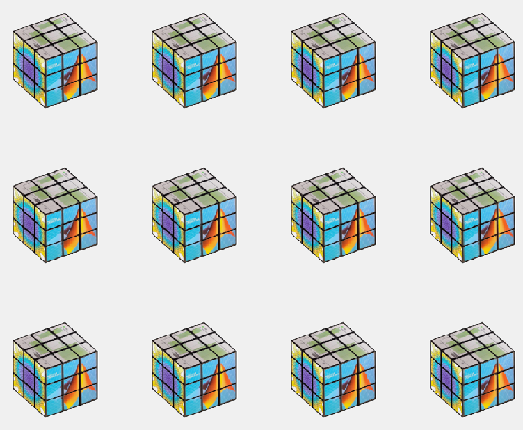
The figure window i really just an interactive image. using getframe()and frame2im() we can quickly turn whatever is shown in the current figure into an image stored in a workspace variable. From here we just need to display that same image multiple times in a sort of array. repmat() in combination with imshow() could have been used here (and would probably have been a bit more flexible in deciding how the cubes are displayed) but I opted for storing the image in a cell array of desired size and using montage() instead.
Most people being character limited in this competition keep everyting to a minimum including the figure windows. Yet I have two of those in my last entry despite only one being shown. As stated in the previous section, surface objects in the workspace is really more of a pointer to the object in the figure, so to keep all my surfaces in between runs I need the figure window containing my surface objects undisturbed. which is why I place the montage in a seperate figure. and display that at the end instead.
An interesting feature *cough* bug *cough* is the swapping between the figure windows that appear in the video generated. This is because of using return as various points in the code in order to skip computations if the move is a 'pause'. The code then does not reach the point where the figure is swaped and montage is made. I thought this to be visually interesting and is therefore dubbing this bug a feature and leaving it in!
Summary:
Multiple cubes were achived by taking the 'image' displayed by the plot window and creating a montage with several of them in a seperate figure window. The swapping between the single and multiple cube view is made by selecting the active figure window before the end of the drawframe call!
Bye for now!
I have yapped on for far too long. Hope you learned something, and thank you all for the kind words and positive response to my entry. This project has been a blast!
Hello! The MathWorks Book Program is thrilled to welcome you to our discussion channel dedicated to books on MATLAB and Simulink. Here, you can:
  • Promote Your Books: Are you an author of a book on MATLAB or Simulink? Feel free to share your work with our community. We’re eager to learn about your insights and contributions to the field.
  • Request Recommendations: Looking for a book on a specific topic? Whether you're diving into advanced simulations or just starting with MATLAB, our community is here to help you find the perfect read.
  • Ask Questions: Curious about the MathWorks Book Program, or need guidance on finding resources? Post your questions and let our knowledgeable community assist you.
We’re excited to see the discussions and exchanges that will unfold here. Whether you're an expert or beginner, there's a place for you in our community. Let's embark on this journey together!
Welcome to the launch of our new blog area, Semiconductor Design and Verification! The mission is to empower engineers and designers in the semiconductor industry by streamlining architectural exploration, optimizing the post-processing of simulations, and enabling early verification with MATLAB and Simulink.
Meet Our Authors
We are thrilled to have two esteemed authors:
@Ganesh Rathinavel and @Cristian Macario Macario have both made significant contributions to the advancement of Analog/Mixed-Signal design and the broader communications, electronics, and semiconductor industries. With impressive engineering backgrounds and extensive experience at leading companies such as IMEC, STMicroelectronics, NXP Semiconductors, LSI Corporation, and ARM, they bring a wealth of knowledge and expertise to our blog. Their work is focused on enhancing MathWorks' tools to better align with industry needs.
What to Expect
The blog will cover a wide range of topics aimed at professionals in the semiconductor field, providing insights and strategies to enhance your design and verification processes. Whether you're looking to streamline your current workflows or explore cutting-edge methodologies, our blog is your go-to resource.
Call to Action
We invite all professionals and enthusiasts in the semiconductor industry to follow our blog posts. Stay updated with the latest trends and insights by subscribing to our blog.
Don’t miss the first post: Accelerating Mixed-Signal Design with Early Behavioral Models, where they explore how early behavioral modeling can accelerate mixed-signal design and enhance system efficiency.
Let's say you have a chance to ask the MATLAB leadership team any question. What would you ask them?
We are thrilled to announce the redesign of the Discussions leaf page, with a new user-focused right-hand column!
Why Are We Doing This?
  • Address Readers’ Needs:
Previously, the right-hand column displayed related content, but feedback from our community indicated that this wasn't meeting your needs. Many of you expressed a desire to read more posts from the same author but found it challenging to locate them.
With the new design, readers can easily learn more about the author, explore their other posts, and follow them to receive notifications on new content.
  • Enhance Authors’ Experience:
Since the launch of the Discussions area earlier this year, we've seen an influx of community members sharing insightful technical articles, use cases, and ideas. The new design aims to help you grow your followers and organize your content more effectively by editing tags. We highly encourage you to use the Discussions area as your community blogging platform.
We hope you enjoy the new design of the right-hand column. Please feel free to share your thoughts and experiences by leaving a comment below.
Marisa
Marisa
최근 활동: 2024년 8월 26일

I am trying to earn my Intro to MATLAB badge in Cody, but I cannot click the Roll the Dice! problem. It simply is not letting me click it, therefore I cannot earn my badge. Does anyone know who I should contact or what to do?
Kindly link me to the Channel Modeling Group.
I read and compreheneded a paper on channel modeling "An Adaptive Geometry-Based Stochastic Model for Non-Isotropic MIMO Mobile-to-Mobile Channels" except the graphical results obtained from the MATLAB codes. I have tried to replicate the same graphs but to no avail from my codes. And I am really interested in the topic, i have even written to the authors of the paper but as usual, there is no reply from them. Kindly assist if possible.
Hello, everyone!
Over the past few weeks, our community has been buzzing with activity, showcasing the incredible depth of knowledge, creativity, and innovation that makes this forum such a vibrant place. Today, we're excited to highlight some of the noteworthy contributions that have sparked discussions, offered insights, and shared knowledge across various topics. Let's dive in!

Interesting Questions

Fatima Majeed brings us a thought-provoking mathematical challenge, delving into inequalities and the realms beyond (e^e). If you're up for a mathematical journey, this question is a must-see!
lil brain tackles a practical problem many of us have faced: efficiently segmenting a CSV file based on specific criteria. This post is not only a query but a learning opportunity for anyone dealing with similar data manipulation challenges.

Popular Discussions

Discover a simple yet effective trick for digit manipulation from goc3. This tip is especially handy for those frequenting Cody challenges or anyone interested in enhancing their number handling skills in MATLAB.
Chen Lin shares an exciting update about the 'Run Code' feature in the Discussions area, highlighting how our community can now directly execute and share code snippets within discussions. This feature marks a significant enhancement in how we interact and solve problems together.

From the Blogs

Connell D`Souza, alongside Team Swarthbeat, explores the cutting-edge application of EEG analysis in predicting neurological outcomes post-cardiac arrest. This blog post offers an in-depth look into the challenges and methodologies of modern medical data analysis.
Mihir Acharya discusses the pivotal role of MATLAB and Simulink in the future of robotics simulation. Through an engaging conversation with industry analyst George Chowdhury, this post sheds light on overcoming simulation challenges and the exciting possibilities that lie ahead.
We encourage everyone to explore these contributions further and engage with the authors and the community. Your participation is what fuels this community's continual growth and innovation.
Here's to many more discussions, discoveries, and breakthroughs together!
📚 New Book Announcement: "Image Processing Recipes in MATLAB" 📚
I am delighted to share the release of my latest book, "Image Processing Recipes in MATLAB," co-authored by my dear friend and colleague Gustavo Benvenutti Borba.
This 'cookbook' contains 30 practical recipes for image processing, ranging from foundational techniques to recently published algorithms. It serves as a concise and readable reference for quickly and efficiently deploying image processing pipelines in MATLAB.
Gustavo and I are immensely grateful to the MathWorks Book Program for their support. We also want to thank Randi Slack and her fantastic team at CRC Press for their patience, expertise, and professionalism throughout the process.
___________

Hello MathWorks Community,

I am excited to announce that I am currently working on a book project centered around Matrix Algebra, specifically designed for MATLAB users. This book aims to cater to undergraduate students in engineering, where Matrix Algebra serves as a foundational element.

Matrix Algebra is not only pivotal in understanding complex engineering concepts but also in applying these principles effectively in various technological solutions. MATLAB, renowned for its powerful computational capabilities, is an excellent tool to explore and implement these concepts, making it a perfect companion for this book.

As I embark on this journey to create a resource that bridges theoretical matrix algebra with practical MATLAB applications, I am looking for one or two knowledgeable individuals who have a firm grasp of both subjects. If you have experience in teaching or applying matrix algebra in engineering contexts and are familiar with MATLAB, your contribution could be invaluable.

Collaborators will help in shaping the content to ensure it is educational, engaging, and technically robust, making complex concepts accessible and applicable for students.

If you are interested in contributing to this project or know someone who might be, please reach out to discuss how we can work together to make this book a valuable resource for engineering students.

Thank you and looking forward to your participation!

First, I felt that the three answers provided by a user in this thread might have been generated by AI. How do you think?
Second, I found that "Responsible usage of generative AI tools, such as ChatGPT, is allowed in MATLAB Answers."
If the answers are indeed AI generated, then the user didn't do "clearly indicating when AI generated content is incorporated".
That leads to my question that how do we enforce the guideline.
I am not against using AI for answers but in this case, I felt the answering text is mentioning all the relevant words but missing the point. For novice users who are seeking answers, this would be misleading and waste of time.
Mathworks has always had quality documentation but in 2023, the documentation quality fell. Will this improve in 2024?
Several of the colormaps are great for a 256 color surface plot, but aren't well optimized for extracting m colors for plotting several independent lines. The issue is that many colormaps have start/end colors that are too similar or are suboptimal colors for lines. There are certainly many workarounds for this, but it would be a great quality of life to adjust that directly when calling this.
Example:
x = linspace(0,2*pi,101)';
y = [1:6].*cos(x);
figure; plot(x,y,'LineWidth',2); grid on; axis tight;
And now if I wanted to color these lines, I could use something like turbo(6) or gray(6) and then apply it using colororder.
colororder(turbo(6))
But my issue is that the ends of the colormap are too similar. For other colormaps, you may get lines that are too light to be visible against the white background. There are plenty of workarounds, with my preference being to create extra colors and truncate that before using colororder.
cmap = turbo(8); cmap = cmap(2:end-1,:); % Truncate the end colors
figure; plot(x,y,'LineWidth',2); grid on; axis tight;
colororder(cmap)
I think it would be really awesome to add some name-argument input pair to these colormaps that can specify the range you want so this could even be done inside the colororder calling if desired. An example of my proposed solution would look something like this:
cmap = turbo(6,'Range',[0.1 0.8]); % Proposed idea to add functionality
Where in this scenario, the resulting colormap would be 6 equally spaced colors that range from 10% to 80% of the total color range. This would be especially nice because you could more quickly modify the range of colors, or you could set the limits regardless of whether you need to plot 3, 6, or 20 lines.