Animation and Model of Automotive Piston
This example shows how to model the motion of an automotive piston by using MATLAB® and Symbolic Math Toolbox™.
Define the motion of an automotive piston and create an animation to model the piston motion.
Step 1: Describe Piston Model
The following figure shows the model of an automotive piston. The moving parts of the piston consist of a connecting rod (red line), a piston crank (green line), and a piston cylinder head (gray rectangle).

Describe the properties of the piston by defining the parameters:
the cylinder stroke length
the piston bore diameter
the length of the connecting rod
the crank radius
the crank angle
Define the origin O of the coordinate system at the crankshaft location. Label the nearest distance between the piston head and the crankshaft location as bottom dead center (BDC). The height of BDC is . Label the farthest distance between the piston head and the crankshaft location as top dead center (TDC). The height of TDC is .
Step 2: Calculate and Plot Piston Height
The following figure is a schematic of the crank and connecting rod.

The height of the piston relative to the origin is Define the piston height as a symbolic function by using the syms function.
syms pistHeight(L,a,theta)
pistHeight(L,a,theta) = a*cos(theta) + sqrt(L^2-a^2*sin(theta)^2);
Assume that the connecting rod length is and the crank radius is . Plot the piston height as a function of the crank angle for one revolution within the interval [0 2*pi].
fplot(pistHeight(150,50,theta),[0 2*pi])
xlabel('Crank angle (rad)')
ylabel('Height (mm)')

The piston head is highest when the piston is at TDC and the crank angle is 0 or 2*pi. The piston head is lowest when the piston is at BDC and the crank angle is pi.
You can also plot the piston height for various values of and . Create a surface plot of the piston height by using the fsurf function. Show the piston height within the interval and .
fsurf(pistHeight(150,a,theta),[30 60 0 2*pi])
xlabel('Crank radius (mm)')
ylabel('Crank angle (rad)')
zlabel('Height (mm)')

Step 3: Calculate and Plot Volume of Piston Cylinder
The length of the combustion chamber is equal to the difference between the TDC location and the piston height. The volume of the piston cylinder can be expressed as .
Define the piston volume as a symbolic function and substitute the expression for with pistHeight.
syms pistVol(L,a,theta,B)
pistVol(L,a,theta,B) = pi*(B/2)^2*(L+a-pistHeight)
pistVol(L, a, theta, B) =
Next, define the values for the following parameters:
the length of the connecting rod
the crank radius
the bore diameter
Plot the piston volume as a function of the crank angle for one revolution within the interval [0 2*pi].
fplot(pistVol(150,50,theta,86),[0 2*pi])
xlabel('Crank angle (rad)')
ylabel('Volume (mm^3)')

The piston volume is smallest when the piston is at TDC and the crank angle is 0 or 2*pi. The piston volume is largest when the piston is at BDC and the crank angle is pi.
Step 4: Evaluate Piston Motion for Changing Angular Speed
Assume the crank rotates at 30 rpm for the first 3 seconds, then steadily increases from 30 to 80 rpm for the next 4 seconds, and then remains at 80 rpm.
Define the angular speed as a function of time by using the piecewise function. Multiply the angular speed by to convert the rotational speed from rpm to rad/sec.
syms t0 t
rpmConv = 2*pi/60;
angVel(t0) = piecewise(t0<=3, 30, t0>3 & t0<=7, 30 + 50/4*(t0-3), t0>7, 80)*rpmConv
angVel(t0) =
Calculate the crank angle by integrating the angular speed using the int function. Assume an initial crank angle of . Compute the integral of the angular speed from 0 to t.
angPos(t) = int(angVel,t0,0,t);
Find the piston height as a function of time by substituting the expression angPos for the crank angle.
H(t) = pistHeight(150,50,angPos)
H(t) =
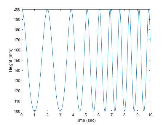
Plot the piston height as a function of time. Notice that the oscillation of the piston height becomes faster between 3 and 7 seconds.
fplot(H(t),[0 10])
xlabel('Time (sec)')
ylabel('Height (mm)')

Step 5: Create Animation of Moving Piston
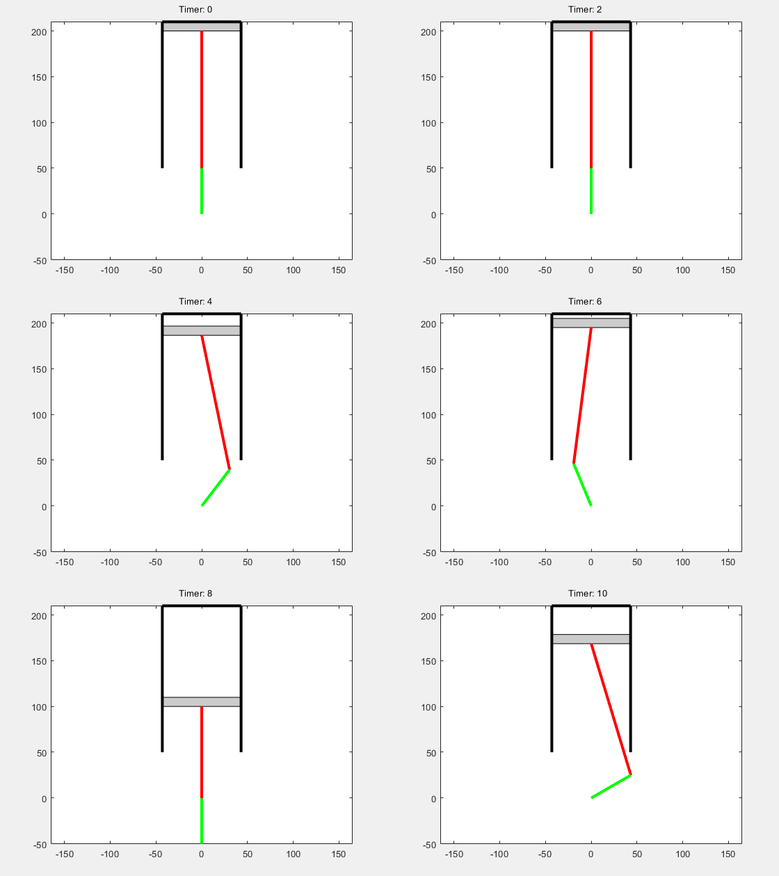
Create an animation of the moving piston given a changing angular speed.
First, create a new figure. Plot the cylinder walls that have fixed locations. Set the x-axis and y-axis to be equal length.
figure;
plot([-43 -43],[50 210],'k','LineWidth',3)
hold on;
plot([43 43],[50 210],'k','LineWidth',3)
plot([-43 43],[210 210],'k','LineWidth',3)
axis equal;
Next, create a stop-motion animation object of the piston head by using the fanimator function. By default, fanimator creates an animation object by generating 10 frames per unit time within the range of t from 0 to 10. Model the piston head as a rectangle with a thickness of 10 mm and variable height H(t). Plot the piston head by using the rectangle function.
fanimator(@rectangle,'Position',[-43 H(t) 86 10],'FaceColor',[0.8 0.8 0.8])
Add the animation objects of the connecting rod and the piston crank. Add a piece of text to count the elapsed time.
fanimator(@(t) plot([0 50*sin(angPos(t))],[H(t) 50*cos(angPos(t))],'r-','LineWidth',3))
fanimator(@(t) plot([0 50*sin(angPos(t))],[0 50*cos(angPos(t))],'g-','LineWidth',3))
fanimator(@(t) text(-25,225,"Timer: "+num2str(t,2)));
hold off;

Use the command playAnimation to play the animation of the moving piston.
