plotResiduals
Syntax
Description
plotResiduals( generates a probability
density plot of the deviance residuals for the multinomial regression model object
mdl)mdl.
plotResiduals( plots on the
axes specified by ax,___)ax instead of the current axes, using any of the
input argument combinations in previous syntaxes.
plotResiduals(___,
specifies additional options using one or more name-value arguments. For example, you can
specify the type of residuals to plot and the colors of the plotted objects.Name=Value)
h = plotResiduals(___)h to modify
the properties of a specific line or patch after you create the plot. For a list of
properties, see Line Properties or Patch Properties.
Examples
Load the fisheriris sample data set.
load fisheririsThe column vector species contains three iris flower species: setosa, versicolor, and virginica. The matrix meas contains four types of measurements for the flowers: the length and width of sepals and petals in centimeters.
Fit a multinomial regression model to predict the iris flower species using the measurements. Display the table of residuals for the fitted model.
mdl = fitmnr(meas,species);
mdl.Residuals
ans=150×3 table
        Raw          Pearson      Deviance
    ___________    ___________    ________

    0    0    0    0    0    0       0
    0    0    0    0    0    0       0
    0    0    0    0    0    0       0
    0    0    0    0    0    0       0
    0    0    0    0    0    0       0
    0    0    0    0    0    0       0
    0    0    0    0    0    0       0
    0    0    0    0    0    0       0
    0    0    0    0    0    0       0
    0    0    0    0    0    0       0
    0    0    0    0    0    0       0
    0    0    0    0    0    0       0
    0    0    0    0    0    0       0
    0    0    0    0    0    0       0
    0    0    0    0    0    0       0
    0    0    0    0    0    0       0
      ⋮
The output shows the raw, Pearson, and deviance residuals for the model.
Generate a probability density plot of the deviance residuals.
plotResiduals(mdl)
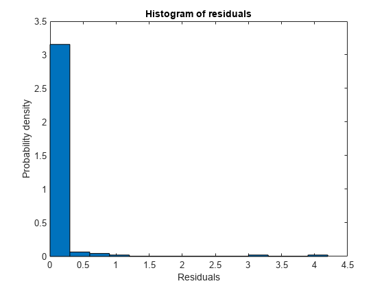
The histogram shows that most of the deviance residuals are small. However, several residuals are greater than one.
Inspect the observations with larger residuals. Sort the residuals from largest to smallest by using the sort function. Use the head function to display the four largest residuals and their corresponding indices.
[r, ind] = sort(mdl.Residuals.Deviance,"descend");
head(r,4)
4.0443
3.1707
1.0378
0.8035
head(ind,4)
    84
   134
    71
   139
The outputs show that observations corresponding to rows 84, 134, and 71 of meas and species have residuals larger than one. Given that most other residuals are close to zero, observations 84, 134, and 71 are most likely outliers.
Load the carbig sample data set.
load carbigThe vectors Displacement, Cylinders, and Model_Year contain data for car engine displacement, number of engine cylinders, and year the car was manufactured, respectively.
Fit a multinomial regression model using Displacement and Cylinders as predictors variables and Model_Year as the response.
mdl = fitmnr([Displacement Cylinders],Model_Year);
To determine whether the residuals are random, generate a lagged plot of the deviance residuals.
plotResiduals(mdl,"lagged")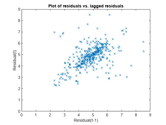
The lagged plot of the deviance residuals shows a cluster of residuals trending toward the top right of the plot. The cluster indicates a mildly positive correlation between the residual for a data point and the residual for the previous data point, suggesting that the residuals might not be random.
Load the carbig sample data set.
load carbigThe vectors Displacement, Cylinders, and Model_Year contain of data for car engine displacement, number of engine cylinders, and year the car was manufactured, respectively.
Fit a nominal multinomial regression model using Displacement and Cylinders as predictors variables and Model_Year as the response.
mdl = fitmnr([Displacement Cylinders],Model_Year);
mdl is a multinomial regression model object that contains the results of fitting a nominal multinomial regression model to the data.
Display the name of the first response category.
mdl.ClassNames(1)
ans =
70
The output shows that the first response category corresponds to cars manufactured in 1970.
To determine whether the raw residuals for cars manufactured in 1970 are randomly distributed, create a probability plot and return a graphics array of the plotted objects. By default, plotResiduals uses the raw residuals for the first response category to create the probability plot.
h = plotResiduals(mdl,"probability",ResidualType="raw")
h =
  2×1 graphics array:

  Line            (main)
  FunctionLine
The output shows the data types for the elements in the graphics array h. The Line element corresponds to the raw residuals. The FunctionLine element corresponds to the line representing the theoretical normal distribution.
Specify the color red for the normal distribution line by modifying the Color property of the second element in h.
h(2).Color = "r"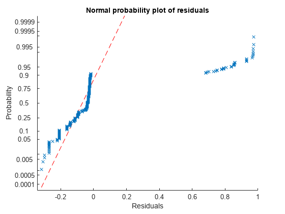
h =
  2×1 graphics array:

  Line            (main)
  FunctionLine
The plot shows that the residuals do not follow the red line, indicating that the raw residuals for cars manufactured in 1970 are not normally distributed.
Input Arguments
Name-Value Arguments
Specify optional pairs of arguments as
Name1=Value1,...,NameN=ValueN, where Name is
the argument name and Value is the corresponding value.
Name-value arguments must appear after other arguments, but the order of the
pairs does not matter.
Example: plotResiduals(mdl,ResidualType="Pearson",ClassToPlot="virginica",FaceColor="m")
generates a magenta histogram for the Pearson residuals of the virginica
response category.
Residuals
Histogram Graphics
Face color, specified as "interp", "flat" an RGB
triplet, a hexadecimal color code, a color name, or a short name.
To designate a single color for all faces, specify FaceColor as an RGB
triplet, a hexadecimal color code, a color name, or a short name.
An RGB triplet is a three-element row vector whose elements specify the intensities of the red, green, and blue components of the color. The intensities must be in the range
[0,1]; for example,[0.4 0.6 0.7].A hexadecimal color code is a character vector or a string scalar that starts with a hash symbol (
#) followed by three or six hexadecimal digits, which can range from0toF. The values are not case sensitive. Thus, the color codes"#FF8800","#ff8800","#F80", and"#f80"are equivalent.
| Color Name | Short Name | RGB Triplet | Hexadecimal Color Code | Appearance |
|---|---|---|---|---|
"red" | "r" | [1 0 0] | "#FF0000" |
|
"green" | "g" | [0 1 0] | "#00FF00" |
|
"blue" | "b" | [0 0 1] | "#0000FF" |
|
"cyan" | "c" | [0 1 1] | "#00FFFF" |
|
"magenta" | "m" | [1 0 1] | "#FF00FF" |
|
"yellow" | "y" | [1 1 0] | "#FFFF00" |
|
"black" | "k" | [0 0 0] | "#000000" |
|
"white" | "w" | [1 1 1] | "#FFFFFF" |
|
"none" | Not applicable | Not applicable | Not applicable | No color |
Here are the RGB triplets and hexadecimal color codes for the default colors MATLAB® uses in many types of plots.
| RGB Triplet | Hexadecimal Color Code | Appearance |
|---|---|---|
[0 0.4470 0.7410] | "#0072BD" |
|
[0.8500 0.3250 0.0980] | "#D95319" |
|
[0.9290 0.6940 0.1250] | "#EDB120" |
|
[0.4940 0.1840 0.5560] | "#7E2F8E" |
|
[0.4660 0.6740 0.1880] | "#77AC30" |
|
[0.3010 0.7450 0.9330] | "#4DBEEE" |
|
[0.6350 0.0780 0.1840] | "#A2142F" |
|
Example: FaceColor="g"
Data Types: single | double | char | string
Face transparency, specified as one of these values:
Scalar in the range
[0,1]— Use uniform transparency across all of the faces. A value of1is fully opaque and0is completely transparent. This option does not use the transparency values in theFaceVertexAlphaDataproperty.'flat'— Use a different transparency for each face based on the values in theFaceVertexAlphaDataproperty. First you must specify theFaceVertexAlphaDataname-value argument as a vector containing one transparency value per face or vertex. The transparency value at the first vertex determines the transparency for the entire face.'interp'— Use interpolated transparency for each face based on the values in theFaceVertexAlphaDataproperty. First you must specify theFaceVertexAlphaDataname-value argument as a vector containing one transparency value per vertex. The transparency varies across each face by interpolating the values at the vertices.
Example: FaceAlpha=0.5
Data Types: single | double | char | string
Line width, specified as a positive value in points, where 1 point = 1/72 of an inch. If the line has markers, then the line width also affects the marker edges.
The line width cannot be thinner than the width of a pixel. If you set the line width to a value that is less than the width of a pixel on your system, the line appears as one pixel wide.
Example: LineWidth=1.5
Data Types: single | double
Note
The graphics properties for histograms listed here are only a subset. For a complete list, see Patch Properties.
Line Graphics
Line color, specified as an RGB triplet, a hexadecimal color code, a color name, or a short name. The default value of [0 0 0] corresponds to black.
For a custom color, specify an RGB triplet or a hexadecimal color code.
An RGB triplet is a three-element row vector whose elements specify the intensities of the red, green, and blue components of the color. The intensities must be in the range
[0,1], for example,[0.4 0.6 0.7].A hexadecimal color code is a character vector or a string scalar that starts with a hash symbol (
#) followed by three or six hexadecimal digits, which can range from0toF. The values are not case sensitive. Therefore, the color codes"#FF8800","#ff8800","#F80", and"#f80"are equivalent.
Alternatively, you can specify some common colors by name. This table lists the named color options, the equivalent RGB triplets, and hexadecimal color codes.
| Color Name | Short Name | RGB Triplet | Hexadecimal Color Code | Appearance |
|---|---|---|---|---|
"red" | "r" | [1 0 0] | "#FF0000" |
|
"green" | "g" | [0 1 0] | "#00FF00" |
|
"blue" | "b" | [0 0 1] | "#0000FF" |
|
"cyan" | "c" | [0 1 1] | "#00FFFF" |
|
"magenta" | "m" | [1 0 1] | "#FF00FF" |
|
"yellow" | "y" | [1 1 0] | "#FFFF00" |
|
"black" | "k" | [0 0 0] | "#000000" |
|
"white" | "w" | [1 1 1] | "#FFFFFF" |
|
"none" | Not applicable | Not applicable | Not applicable | No color |
Here are the RGB triplets and hexadecimal color codes for the default colors MATLAB uses in many types of plots.
| RGB Triplet | Hexadecimal Color Code | Appearance |
|---|---|---|
[0 0.4470 0.7410] | "#0072BD" |
|
[0.8500 0.3250 0.0980] | "#D95319" |
|
[0.9290 0.6940 0.1250] | "#EDB120" |
|
[0.4940 0.1840 0.5560] | "#7E2F8E" |
|
[0.4660 0.6740 0.1880] | "#77AC30" |
|
[0.3010 0.7450 0.9330] | "#4DBEEE" |
|
[0.6350 0.0780 0.1840] | "#A2142F" |
|
Example: Color="blue"
Example: Color=[0 0 1]
Example: Color="#0000FF"
Data Types: single | double | char | string
Line style, specified as one of the options listed in this table.
| Line Style | Description | Resulting Line |
|---|---|---|
"-" | Solid line |
|
"--" | Dashed line |
|
":" | Dotted line |
|
"-." | Dash-dotted line |
|
"none" | No line | No line |
Example: LineStyle="--"
Data Types: char | string
Marker symbol, specified as one of the values listed in this table. By default, the object does not display markers. Specifying a marker symbol adds markers at each data point or vertex.
| Marker | Description | Resulting Marker |
|---|---|---|
"o" | Circle |
|
"+" | Plus sign |
|
"*" | Asterisk |
|
"." | Point |
|
"x" | Cross |
|
"_" | Horizontal line |
|
"|" | Vertical line |
|
"square" | Square |
|
"diamond" | Diamond |
|
"^" | Upward-pointing triangle |
|
"v" | Downward-pointing triangle |
|
">" | Right-pointing triangle |
|
"<" | Left-pointing triangle |
|
"pentagram" | Pentagram |
|
"hexagram" | Hexagram |
|
"none" | No markers | Not applicable |
Example: Marker="x"
Data Types: char | string
Note
The graphics properties for lines listed here are only a subset. For a complete list, see Line Properties.